Week 2: Workflow

.R & .qmd, Projects, Read Data

Joe Nese

University of Oregon
Fall 2025

Hex stickers!

Let’s give Xinyu a hex sticker!

Hex stickers!

And let’s give Cheyna a hex sticker for sharing today!

Share out

Custom Editor theme!

Housekeeping

  • Slides as pdf
  • Screenshots
    • Something to show you completed the Codecademy lesson in its entirety
    • Only responsible for the free Lessons

Workflow

Week 2

Agenda

  • Project Oriented Workflow
    • RStudio Projects
    • File paths
    • Reading in data
    • Scripts (.R & .qmd)
    • Loading packages
  • Looking at data
  • The pipe |>
    • also %>%

Learning Objectives

  • Open an RStudio Project
  • Understand file paths
  • Learn two ways to read data
  • Establish good workflow habits

RStudio Projects

RStudio Projects (.Rproj)

An RStudio project - .Rproj - is basically a folder to house all the files for your project

  • scripts
  • products
  • data
  • figures

RStudio Projects (.Rproj)

Advantages

  • Work with several projects at the same time (several projects open)
    • these are self-contained!
  • Can save the history of your commands after quitting
  • Can specify version control system (e.g., Git)
  • Previously edited code tabs are restored upon opening
  • The current working directory is set to the project directory

What’s a working directory?

Where you’re at on your computer

  • the folder location
  • Quick check-in: does this make sense?

You can change your working directory with setwd("path/to/files")

BUT I strongly urge you to avoid that

Instead, we’re going to use RStudio Projects and the {here} package

  • See where you’re currently at by looking at the top of the console
  • Or run getwd() in the console

What’s different with .Rproj?

Your working directory is immediately wherever your .Rproj project is located

This is true for whoever is accessing the project

Use the {here} package to specify paths

  • You can read/save data (and figures, products, etc.) which we’ll talk about more later

Best practices

here()

  • works for anyone who uses the script
  • share it out with no code editing
  • easy to work on other projects with different directories

Session > Restart R

Restart the R session

  • Create a fresh R process
  • Deletes all objects
  • Packages will need to be re-loaded
  • Resets any code-enables options
  • Ensures script is self-contained

Project Oriented Workflow

Write every script assuming it will be run in a fresh R process

  1. Do not save .RData when you quit R and don’t load .RData when you start R

Week 1: Tools 🡆 Global Options 🡆 General

Workspace

  • Restore .RData into workspace at startup” – Uncheck
  • Save workspace to .RData on exit:” – Never

Project Oriented Workflow

Write every script assuming it will be run in a fresh R process

  1. Daily work habit:
  • Restart R very often and re-run your developing script from the top
  • Use the RStudio menu item
    • Session > Restart R (Ctrl/Command + Shift + F10)

Workflow

Let’s start by making a new project

Typical workflow

  1. Make a new .RProj

  2. Add folders

    • “data”
    • “scripts”
  3. Add data

  4. Create scripts

  5. Load packages

RStudio Project

1. Make a new .RProj

File > New Project…

or - upper right of RStudio by the R cube

⬇️ > New Project…

1. Make a new .RProj

Let’s name it: “my_first_project”

  • notice the naming convention
    • no caps
    • no spaces
    • no special characters (e.g., ?, !, ", #)
    • _” and “-” are ok

Choose a location for it

  • An .RProj will need its own folder, with no other projects in it!
  • Projects in Dropbox often lead to unexpected occurences

I’ll just save “my_first_project” to my desktop

demo

Organize

2. Create folders

Let’s make two folder in different ways (either is fine)

“data”

  • where we will store all our project-related data
  • let’s create that in Rstudio

“scripts”

  • where we will hold all our scripts (.R or .Rmd or .qmd files)
  • let’s create that in the folder on our machine

demo

Reading Data

Dowload data

Let’s save the following data files into our project “data” folder

(go here to download)

  1. ecls-k_samp.sav
  2. Fatality.txt
  3. Project_Reads_Scores.csv

Let’s see files are in our “data” folder

  • You can list.files("path/to/files") to see the contents of your project directory (i.e., what your computer “sees”)

  • You can also use the Files tab in RStudio

  • Use here() to access data or any file in your project
  • here() is simply a function to print a path
    • list.files(here("data")) . . .

demo

Reading data into R

You just need two things:

  1. where the dataset it located

This is most often just a path on you machine

  1. package::function() to read the data

We’ll be talking about two data reading packages

  • {rio}
  • {readr}

We’ll use the {here} package

{here} uses the top-level directory of a project to easily build paths to files

  • Allows you to worry about paths a little less
  • Helps reproducibility
  • Your final project!

Think of here() simply as a function to print a path name

A path can be the lcoation of your data

path = lcoation

{here}

Think of here() simply as a function to print a path name

First, install/load {here} the package

# In the console: 
# install.packages("here")
# Then, load the package

library(here)

{here}

Think of here() simply as a function to print a path name

Run this code in your project (console is fine)

here()
[1] "C:/Users/jnese/Desktop/BRT/Teaching/1_Intro-Data-Science/intro-DS-R_fall-2025"

This is the “top level” directory of my project

{here}

Think of here() simply as a function to print a path

Run this code in your project (console is fine)

here()
[1] "C:/Users/jnese/Desktop/BRT/Teaching/1_Intro-Data-Science/intro-DS-R_fall-2025"

This is the path to the project directory

here("data")
[1] "C:/Users/jnese/Desktop/BRT/Teaching/1_Intro-Data-Science/intro-DS-R_fall-2025/data"

This is the path to the “data” folder in our project directory

{here}

Think of here() simply as a function to print a path

here()
[1] "C:/Users/jnese/Desktop/BRT/Teaching/1_Intro-Data-Science/intro-DS-R_fall-2025"
here("data")
[1] "C:/Users/jnese/Desktop/BRT/Teaching/1_Intro-Data-Science/intro-DS-R_fall-2025/data"

Question: What was the difference in the output between these?

Question: What will the following produce?

here("data", "ecls-k_samp.sav")
[1] "C:/Users/jnese/Desktop/BRT/Teaching/1_Intro-Data-Science/intro-DS-R_fall-2025/data/ecls-k_samp.sav"

Reading Data

{rio}

  • {rio} is a wrapper around many different packages that import/export data in different formats

  • Great package

  • Most of the time “it just works” regardless of the source file type

    • this might not impress you, but it really should!
    • any package that turns a complex task into a simple procedure that “just works” is invaluable

rio::import()

import(file, format, setclass, …)

file = character string naming a file

format = (optional) character string of file format; e.g., "," for comma-separated values

setclass = (optional) character vector specifying one or more classes to set on the import. Default is "data.frame". We would probably prefer "tbl_df" for a tibble

rio::import()

import(file)

file = character string naming a file

3a. Read in data

Try it!

library(rio)
#library(tidyverse)

# .sav
eclsk <- import(here("data", "ecls-k_samp.sav"), setclass = "tbl_df")

# Use `as_tibble` instead of `setclass = "tbl_df"`

# .txt
fatality <- import(here("data", "Fatality.txt")) |> 
  as_tibble()

#.csv
exam1 <- import(here("data", "Project_Reads_Scores.csv")) |> 
  as_tibble()

You can even read directly from the web 😲

Fatality.txt

import("https://raw.githubusercontent.com/jnese/intro-DS-R_fall-2025/master/data/Fatality.txt",
       setclass = "tbl_df")
# A tibble: 336 × 10
   state  year mrall beertax  mlda jaild comserd vmiles unrate perinc
   <int> <int> <dbl>   <dbl> <dbl> <chr> <chr>    <dbl>  <dbl>  <dbl>
 1     1  1982  2.13   1.54   19   no    no        7.23  14.4  10544.
 2     1  1983  2.35   1.79   19   no    no        7.84  13.7  10733.
 3     1  1984  2.34   1.71   19   no    no        8.26  11.1  11109.
 4     1  1985  2.19   1.65   19.7 no    no        8.73   8.90 11333.
 5     1  1986  2.67   1.61   21   no    no        8.95   9.80 11662.
 6     1  1987  2.72   1.56   21   no    no        9.17   7.80 11944 
 7     1  1988  2.49   1.50   21   no    no        9.67   7.20 12369.
 8     4  1982  2.50   0.215  19   yes   yes       6.81   9.90 12309.
 9     4  1983  2.27   0.206  19   yes   yes       6.59   9.10 12694.
10     4  1984  2.83   0.297  19   yes   yes       6.71   5    13266.
# ℹ 326 more rows

Write data

Save data just as easily with rio::export()

You need two things:

  1. What to export?
  2. Where to export?

export(x, file, format, …)

x = data frame (tibble) to be written into a file

file = character string naming a file

export(fatality, here("data", "exam1.sav"))

export(fatality, here("data", "exam1.txt"))

export(fatality, here("data", "exam1.dta"))

convert()

Another really useful feature is convert(), which just takes a file of one type and converts it to another

Say your advisor uses SPSS 😐, but their colleague uses Stata 😐, and you use R 😎

Just run one line of code!

convert(in_file, out_file, …)

in_file = character string naming an input file

out_file = character string naming an output file

convert(here(“data”, ecls-k_samp.sav), here(“data”, ecls-k_samp.txt))

How is this all working?

{rio} wraps a variety of faster, more modernized packages than those provided by base R

  • {data.table} for delimited formats
  • {readxl} and {openxlsx} for reading and writing Excel workbooks
  • data.table::fread() for text-delimited files to automatically determine the file format regardless of the extension
    • also very fast

Again, import() “just works”

Maintaining data “labels”

Question: How many of you or your colleagues use SPSS or Stata?

and/or: How many of you use Qualtrics?

In SPSS, Stata, & Qualtrics numeric data are often encoded with labels

For SAS, Stata, and SPSS files use {haven}

{haven} allow you to transform the data into the character/factor version

{haven} store metadata from rich file formats (SPSS, Stata, etc.) in variable-level attributes in a consistent form regardless of file type or underlying import function

  • rio::characterize() converts a single variable or all variables in the data that have label attributes into character vectors
  • rio::factorize() does the same but returns factor variables

This is very important for several of your homeworks!

eclsk |>
  select(child_id, k_type:sex) 
# A tibble: 984 × 4
   child_id k_type school_type   sex
   <chr>     <dbl>       <dbl> <dbl>
 1 0842021C      1           0     0
 2 0905002C      1           1     0
 3 0150012C      1           1     1
 4 0556009C      1           1     1
 5 0089013C      1           0     0
 6 1217001C      0           0     1
 7 1092008C      0           0     1
 8 0083007C      1           0     0
 9 1091005C      0           1     0
10 2006006C      1           1     0
# ℹ 974 more rows

eclsk |>
  characterize() |>
  select(child_id, k_type:sex) 
# A tibble: 984 × 4
   child_id k_type   school_type sex   
   <chr>    <chr>    <chr>       <chr> 
 1 0842021C full-day public      male  
 2 0905002C full-day private     male  
 3 0150012C full-day private     female
 4 0556009C full-day private     female
 5 0089013C full-day public      male  
 6 1217001C half-day public      female
 7 1092008C half-day public      female
 8 0083007C full-day public      male  
 9 1091005C half-day private     male  
10 2006006C full-day private     male  
# ℹ 974 more rows

{readr}

  • Great package; most of the time “it just works” regardless of the source file type
  • Loads with {tidyverse}
  • Default loads data as a tibble
    • this is nice!

read_csv()

You just need one thing:

  1. where the data is located

read_csv(file, …)

file = a path to a file, a connection, or literal data (either a single string or a raw vector)

And how do we get a path string?

with the here() function

read_csv(here("path", "to", "data.csv"))

3b. Read in data

Try it!

library(tidyverse)

# read_table() for space separated data
fatality <- read_table(here("data", "Fatality.txt")) 

#read_csv(), the one I most often use
exam1 <- read_csv(here("data", "Project_Reads_Scores.csv"))

# read directly from the web, in this case a .csv
web <- read_csv("https://github.com/datalorax/ncme_18/raw/master/data/pubschls.csv")

write_*()

Save data just as easily with write_*()

You need two things:

  1. What to export?
  2. Where to export?

write_csv(x, file, …)

x = data frame (tibble) to be written into a file

file = character string naming a file to write to

Basically

write_*(what, "where")

write_csv(exam1, here("data", "exam1.csv"))

Scripts

.R

.R is R script (code) file

File > New File > R Script

  • Everything is code
  • Text - comments! - need to begin with “#
    • Comments are a great habit!
    • Use them to document the what & why of your code

Run code

  • Ctrl/Command + Enter
  • Highlight specific code, Ctrl/Command + Enter
  • Put mouse on line, Ctrl/Command + Enter, and it will execute the all connected (piped) code

demo

Quick Peek

What is Quarto?

  • an open-source scientific and technical publishing system
  • create dynamic content with Python, R, Julia, and Observable.
  • publish reproducible, production quality articles, presentations, websites, blogs, and books in HTML, PDF, MS Word, ePub, etc.
  • include equations, citations, crossrefs, figure panels, callouts, advanced layout, etc.
  • a multi-language, next generation version of R Markdown (from Posit)
  • includes many built in output formats (and options for customizing each)
  • has native features for special project types like Websites, Books, and Blogs (rather than relying on external packages)

Why Quarto?

  • Reproducibility: reproducible workflow
    • Code + output + prose together
    • Syntax highlighting FTW!
    • Familiar-feeling authoring with the visual editor without having to learn a bunch of new markdown syntax
  • Efficiency: consistent formatting
  • Extendability: Use with Python, and Julia, and Observable, and more

.qmd

.qmd is a document format file that combines code AND prose

  • File > New File > Quarto document…

Code goes into “code chunks”

```{r}
#| eval: false
# comment

data |> 
  select(id, read, math)
```

Prose goes outside the code chunks

demo

.R & .qmd

  • Both are great
  • Serve different purposes

Organization tip

  • .qmd with headers
  • .R with # Header ----

demo

Packages

Packages

First the package must be installed on your machine

install.packages(“package_name”)

  • you will only need to do this the first time you want to use the package
  • never keep this code line (just run it in the console!)
  • notices the quotes around the package name
  • never keep this code line

Any time you want to use a package it should be loaded

library(package_name)

  • you will do this each time you use the package in your scripts
  • notices no quotes around the package name

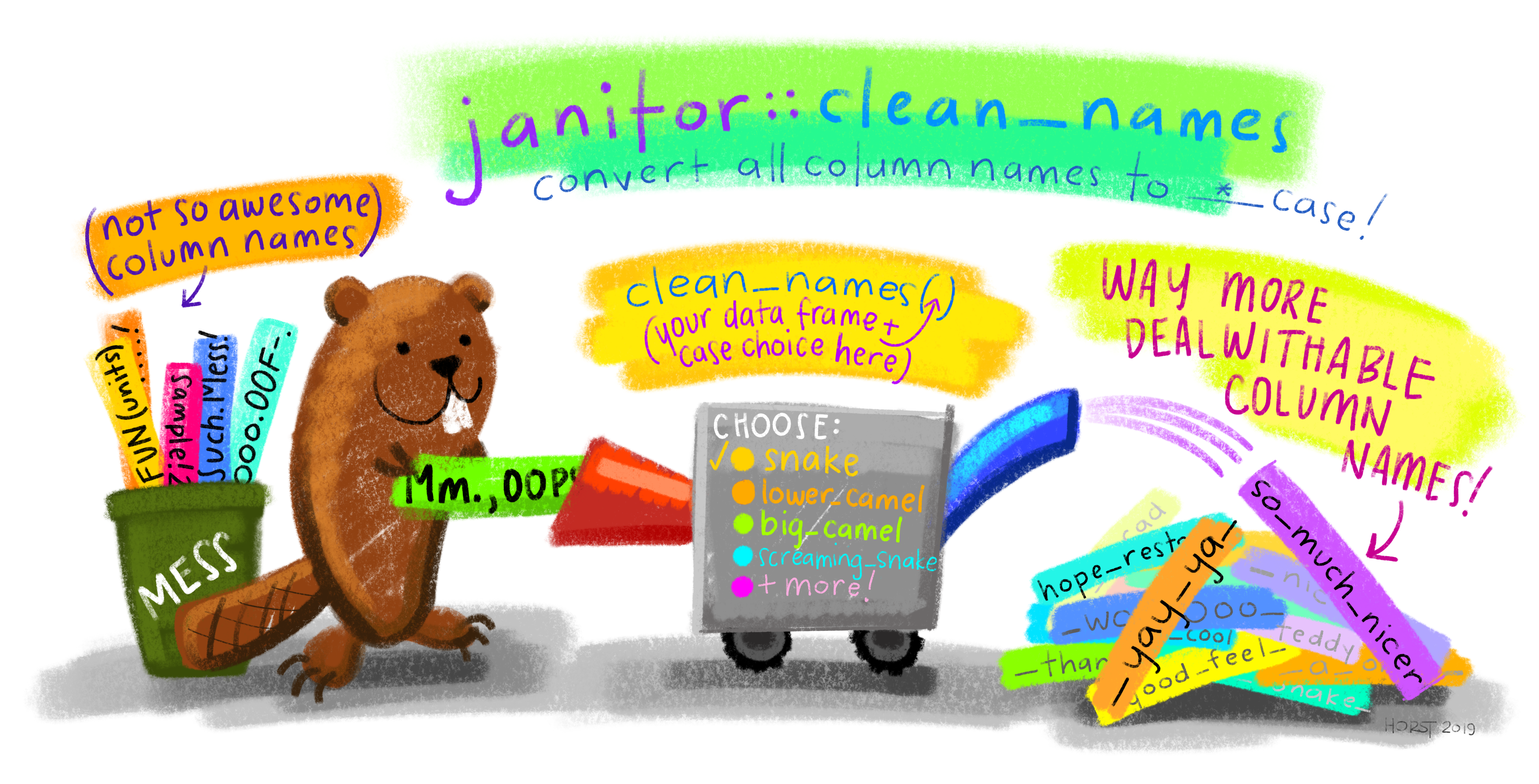
{janitor}

A fantastic package!

  • remove_empty_rows()
  • remove_empty_cols()
  • excel_numeric_to_date()
    • changes numeric dates imported from Excel to actual dates
  • tabyl()
    • frequency table with n and %
  • clean_names()
    • styles column names (NOT data itself) with “snake_case”
      • lower case and underscore between words
    • can choose a different “*_case

Let’s put it all together

New script

Let’s work within the “my_first_project” .RProj

  1. Open a new Quarto document

demo

New script

Let’s work within the “my_first_project” .RProj

  1. Clean it up
    1. Modify the YAML
    2. Save the file as “practice.qmd” in the scripts folder
    3. Render!

demo

New script

  • Opens with a template
  • Going forward with .qmd…
    1. you can delete everything in the template, or
    2. you can open an empty .qmd document

but do one of these

Working with data

  1. What packages will we use?
  • library(here) - where the data is located
  • library(rio) - read the data into R
  • library(janitor) - clean the variable names in the data
  • library(tidyverse) - clean the data

Working with data

  1. Read in the Penguins.csv data
  • Let’s name the data “penguins
  • Three options, choose one
# rio::import()
penguins <- import(here("data", "Penguins.csv"), setclass = "tbl_df")

penguins <- import(here("data", "Penguins.csv"))

# readr::read_csv()
penguins <- read_csv(here("data", "Penguins.csv")) 

What do our data look like?

penguins
# A tibble: 344 × 8
   Species Island    `Bill Length (mm)` `Bill Depth (mm)` `Flipper Length (mm)`
   <chr>   <chr>                  <dbl>             <dbl>                 <dbl>
 1 Adelie  Torgersen               39.1              18.7                   181
 2 Adelie  Torgersen               39.5              17.4                   186
 3 Adelie  Torgersen               40.3              18                     195
 4 Adelie  Torgersen               NA                NA                      NA
 5 Adelie  Torgersen               36.7              19.3                   193
 6 Adelie  Torgersen               39.3              20.6                   190
 7 Adelie  Torgersen               38.9              17.8                   181
 8 Adelie  Torgersen               39.2              19.6                   195
 9 Adelie  Torgersen               34.1              18.1                   193
10 Adelie  Torgersen               42                20.2                   190
# ℹ 334 more rows
# ℹ 3 more variables: `Body Mass (g)` <dbl>, Sex <chr>, Year <dbl>

Or use View() to take a look at the full data in RStudio

View(penguins)

or click on the object name in your RStudio Environment

janitor::clean_names()

# re-assign the "reads" object by reading the data in again
penguins <- read_csv(here("data", "Penguins.csv")) |> 
  clean_names()

# or just work with the existing "penguins" object
penguins <- penguins |> 
  clean_names()

Looking at the data structure

structure

str(penguins)
spc_tbl_ [344 × 8] (S3: spec_tbl_df/tbl_df/tbl/data.frame)
 $ species          : chr [1:344] "Adelie" "Adelie" "Adelie" "Adelie" ...
 $ island           : chr [1:344] "Torgersen" "Torgersen" "Torgersen" "Torgersen" ...
 $ bill_length_mm   : num [1:344] 39.1 39.5 40.3 NA 36.7 39.3 38.9 39.2 34.1 42 ...
 $ bill_depth_mm    : num [1:344] 18.7 17.4 18 NA 19.3 20.6 17.8 19.6 18.1 20.2 ...
 $ flipper_length_mm: num [1:344] 181 186 195 NA 193 190 181 195 193 190 ...
 $ body_mass_g      : num [1:344] 3750 3800 3250 NA 3450 ...
 $ sex              : chr [1:344] "male" "female" "female" NA ...
 $ year             : num [1:344] 2007 2007 2007 2007 2007 ...
 - attr(*, "spec")=
  .. cols(
  ..   Species = col_character(),
  ..   Island = col_character(),
  ..   `Bill Length (mm)` = col_double(),
  ..   `Bill Depth (mm)` = col_double(),
  ..   `Flipper Length (mm)` = col_double(),
  ..   `Body Mass (g)` = col_double(),
  ..   Sex = col_character(),
  ..   Year = col_double()
  .. )
 - attr(*, "problems")=<externalptr> 

Looking at the data properties

dimensions (rows \(\times\) columns)

dim(penguins)
[1] 344   8

number of rows or number of columns

nrow(penguins)
[1] 344
ncol(penguins)
[1] 8

Another cool package {skimr}

library(skimr)

skim(penguins)
Data summary
Name penguins
Number of rows 344
Number of columns 8
_______________________
Column type frequency:
character 3
numeric 5
________________________
Group variables None

Variable type: character

skim_variable n_missing complete_rate min max empty n_unique whitespace
species 0 1.00 6 9 0 3 0
island 0 1.00 5 9 0 3 0
sex 11 0.97 4 6 0 2 0

Variable type: numeric

skim_variable n_missing complete_rate mean sd p0 p25 p50 p75 p100 hist
bill_length_mm 2 0.99 43.92 5.46 32.1 39.23 44.45 48.5 59.6 ▃▇▇▆▁
bill_depth_mm 2 0.99 17.15 1.97 13.1 15.60 17.30 18.7 21.5 ▅▅▇▇▂
flipper_length_mm 2 0.99 200.92 14.06 172.0 190.00 197.00 213.0 231.0 ▂▇▃▅▂
body_mass_g 2 0.99 4201.75 801.95 2700.0 3550.00 4050.00 4750.0 6300.0 ▃▇▆▃▂
year 0 1.00 2008.03 0.82 2007.0 2007.00 2008.00 2009.0 2009.0 ▇▁▇▁▇

The pipe operator (|>)

  • The |> operator (Super + Shift + M)
    • inserts the input as the first argument in the next function
  • To start, you can read it as “then”
  • It is crucial for work in the {tidyverse}

The pipe operator (|>)

  • Get a frequency count

With the {tidyverse}

penguins |> 
  count(species)
# A tibble: 3 × 2
  species       n
  <chr>     <int>
1 Adelie      152
2 Chinstrap    68
3 Gentoo      124

Or with {janitor}

penguins |> 
  tabyl(species)
   species   n   percent
    Adelie 152 0.4418605
 Chinstrap  68 0.1976744
    Gentoo 124 0.3604651

Let’s look at ?count and ?tabyl

demo

Why use |>

Chaining arguments is efficient and easy to read

penguins |> 
  filter(species == "Adelie",
         bill_length_mm > 40) |> 
  select(island, bill_length_mm, body_mass_g) |> 
  arrange(bill_length_mm) 
# A tibble: 51 × 3
   island    bill_length_mm body_mass_g
   <chr>              <dbl>       <dbl>
 1 Biscoe              40.1        4300
 2 Torgersen           40.2        3450
 3 Dream               40.2        3975
 4 Dream               40.2        3400
 5 Torgersen           40.3        3250
 6 Dream               40.3        4350
 7 Biscoe              40.5        3200
 8 Biscoe              40.5        3950
 9 Biscoe              40.6        3550
10 Biscoe              40.6        3800
# ℹ 41 more rows

Why use |>

Chaining arguments is efficient and easy to read

penguins |> 
  filter(species == "Adelie",
         bill_length_mm > 40) |>
  select(island, bill_length_mm, body_mass_g) |> 
  arrange(bill_length_mm) 

Equivalent to:

arrange(select(filter(penguins, species == "Adelie", bill_length_mm > 40), island, bill_length_mm, body_mass_g), bill_length_mm)

|>

The |> works so well in the {tidyverse} because the first argument in (nearly) all functions is the dataframe (tibble)


So you don’t need to name the data each time

So this:

penguins |> 
  count(sex)
# A tibble: 3 × 2
  sex        n
  <chr>  <int>
1 female   165
2 male     168
3 <NA>      11

Is equivalent to this:

count(penguins, sex)
# A tibble: 3 × 2
  sex        n
  <chr>  <int>
1 female   165
2 male     168
3 <NA>      11

Next time

Homework notes

Script on website

  • Download Homework 1 from the course Assignments page
  • Work with this .qmd file

Submit a rendered .html file to Canvas

  • Assignments > Homeworks > HW 1

let’s take a look!

Before next class