Week 2: Intro to Base `R` Iterations

& Lab 1

Joe Nese

University of Oregon
Spring 2026

Base `R` Iterations &
Lab 1

Week 2

Agenda

For loops
Apply family of loops
- lapply()
- sapply()
- vapply()
- apply() (briefly)
Lab 1 (🤞)

Learning objectives

Understand the basics of what it means to loop through a vector
Begin to recognize use cases
Be able to apply basic for loops and write their equivalents with lapply

`for` loops

Basic overview `for` loops

a <- letters[1:26]
a

 [1] "a" "b" "c" "d" "e" "f" "g" "h" "i" "j" "k" "l" "m" "n" "o" "p" "q" "r" "s"
[20] "t" "u" "v" "w" "x" "y" "z"

for(i in 1:5){
    print(a[i])
}

[1] "a"
[1] "b"
[1] "c"
[1] "d"
[1] "e"

Note these are five different character scalars (atomic vectors of length one)

It is NOT a single vector

Creating indexes

You will commonly see code like this:

for(i in 1:nrow(df)) {some_function}

Instead, use seq_along() or seq_len()

`seq_*`

seq_along()
- takes a vector argument
- creates an index from 1 to the length of the vector provided
seq_len()
- takes a single positive integer argument
- creates an index from 1 to that integer

x <- c(3, 2.6, 8)

seq_along(x)

[1] 1 2 3

seq_len(length(x))

[1] 1 2 3

Why are these preferable?

Avoids the `length` of `0` problem

: works with both increasing and decreasing sequences, which is problematic

means <- c()

length(means)

[1] 0

1:length(means)

[1] 1 0

Avoids the `length` of `0` problem

X <- 1:10
N <- length(X)

i <- 1

: method

X[(i+1):N]

[1]  2  3  4  5  6  7  8  9 10

X[1:(i-1)]

[1] 1

seq_len() method

X[-seq_len(i)]

[1]  2  3  4  5  6  7  8  9 10

X[seq_len(i-1)]

integer(0)

Another example

Try this

means <- c()
out <- rep(NA, length(means))
out

logical(0)

for (i in 1:length(means)) {
  out[i] <- rnorm(10, means[i])
}

Error in `rnorm()`:
! invalid arguments

seq_* version

for (i in seq_along(means)) {
  out[i] <- rnorm(10, means[i])
}

Basically, the loop is just not executed

Another `for` loop example

Simulate tossing a coin, record results

For a single toss

sample(c("Heads", "Tails"), 1)

[1] "Tails"

For multiple tosses, first allocate a vector with length equal to the number of iterations (here, 10)

(result <- rep(NA, 10))

 [1] NA NA NA NA NA NA NA NA NA NA

Next, run the trial \(n\) times, storing the result in your pre-allocated vector

for(i in seq_along(result)) {
    result[i] <- sample(c("Heads", "Tails"), 1)
}

Wait, what?

result

 [1] "Heads" "Heads" "Heads" "Tails" "Tails" "Heads" "Tails" "Heads" "Heads"
[10] "Heads"

Growing vectors

ALWAYS pre-allocate a vector for storage before running a for loop
Contrary to some opinions you may see out there, for loops are not actually slower than lapply, etc., provided the for loop is written well
This primarily means not growing a vector

Growing vector example

100,000 (1e5) coin flips by growing a vector

library(tictoc)

set.seed(3000)
tic()
not_allocated <- sample(c("Heads", "Tails"), 1)
for(i in seq_len(1e5 - 1)) {
    not_allocated <- c(
      not_allocated, 
      sample(c("Heads", "Tails"), 1)
     )
  
}
toc()

61.15 sec elapsed

Pre-allocated vector example

Exactly the same thing with pre-allocated vector

set.seed(3000)
tic()
allocated <- rep(NA, 1e5)
for(i in seq_len(1e5)) {
    allocated[i] <- sample(c("Heads", "Tails"), 1)
}
toc()

1.22 sec elapsed

Result

The result is the same, regardless of the approach (notice I forced the random number generator to start at the same place in both samples)

identical(not_allocated, allocated)

[1] TRUE

But speed is obviously NOT identical

You try

Base R comes with letters and LETTERS

Make an alphabet of upper/lower case
- For example, create “Aa” with
  paste0(LETTERS[1], letters[1])
Write a for loop for all letters

Don’t look ahead!

Answer

alphabet <- rep(NA, length(letters))

for(i in seq_along(alphabet)) {
    alphabet[i] <- paste0(LETTERS[i], letters[i])
}

Where is it?

alphabet

 [1] "Aa" "Bb" "Cc" "Dd" "Ee" "Ff" "Gg" "Hh" "Ii" "Jj" "Kk" "Ll" "Mm" "Nn" "Oo"
[16] "Pp" "Qq" "Rr" "Ss" "Tt" "Uu" "Vv" "Ww" "Xx" "Yy" "Zz"

Another example

Say we wanted to simulate 100 cases from a random normal (rnorm()) distribution, where we varied the standard deviation in increments of 0.2, ranging from 1 to 5
- Maybe this is a relatable example; if not, that’s okay - focus on the process

First, specify a vector of standard deviations

increments <- seq(1, 5, by = 0.2)
increments

 [1] 1.0 1.2 1.4 1.6 1.8 2.0 2.2 2.4 2.6 2.8 3.0 3.2 3.4 3.6 3.8 4.0 4.2 4.4 4.6
[20] 4.8 5.0

Next, allocate a vector. There are many ways I could store this result (data frame, matrix, list). I’ll do it in a list.

simulated <- vector("list", length(increments))

Look at our vector

str(simulated)

List of 21
 $ : NULL
 $ : NULL
 $ : NULL
 $ : NULL
 $ : NULL
 $ : NULL
 $ : NULL
 $ : NULL
 $ : NULL
 $ : NULL
 $ : NULL
 $ : NULL
 $ : NULL
 $ : NULL
 $ : NULL
 $ : NULL
 $ : NULL
 $ : NULL
 $ : NULL
 $ : NULL
 $ : NULL

Write a `for` loop

for(i in seq_along(simulated)) {
    simulated[[i]] <- rnorm(100, 0, increments[i]) 
}

note use of [[ above

Now look at our vector

str(simulated)

List of 21
 $ : num [1:100] 0.113 -1.034 1.039 0.75 -0.762 ...
 $ : num [1:100] -0.478 0.899 -1.879 -0.562 1.329 ...
 $ : num [1:100] -1.6934 -1.3552 -2.413 -0.5348 0.0318 ...
 $ : num [1:100] 1.084 -0.822 -1.952 1.2 0.265 ...
 $ : num [1:100] 0.64 -0.04 -0.715 -0.309 0.494 ...
 $ : num [1:100] -3.98 -2.165 0.488 -2.217 -2.08 ...
 $ : num [1:100] -1.691 -0.576 -0.239 3.253 0.777 ...
 $ : num [1:100] 2.975 0.673 2.041 -2.141 1.652 ...
 $ : num [1:100] -1.447 -2.445 -4.24 0.148 -0.355 ...
 $ : num [1:100] 4.71 -3.84 -3.27 5.42 1.67 ...
 $ : num [1:100] 0.115 -2.412 -1 -2.307 -0.332 ...
 $ : num [1:100] 0.727 1.451 -0.163 1.078 -5.881 ...
 $ : num [1:100] 0.79 -4.756 -0.829 -2.805 -2.242 ...
 $ : num [1:100] 1.883 0.458 1.318 5.461 2.404 ...
 $ : num [1:100] 3.53 1.14 -10.58 7.69 -6.24 ...
 $ : num [1:100] -5.903 3.891 2.005 -0.756 -6.651 ...
 $ : num [1:100] -1.875 3.626 -0.837 -4.227 0.305 ...
 $ : num [1:100] 6.78 -6.19 -12.4 -1.79 -3.45 ...
 $ : num [1:100] 6.04 -1.47 -1.9 5.37 3.16 ...
 $ : num [1:100] 3.976 6.997 1.454 0.294 1.205 ...
 $ : num [1:100] 4.02 1.46 -1.78 8.73 -8.37 ...

List/data frame

Remember, if all the vectors of our list are the same length, it can be transformed into a data frame

First, let’s provide meaningful names

names(simulated) <- paste0("sd_", increments)
str(simulated)

List of 21
 $ sd_1  : num [1:100] 0.113 -1.034 1.039 0.75 -0.762 ...
 $ sd_1.2: num [1:100] -0.478 0.899 -1.879 -0.562 1.329 ...
 $ sd_1.4: num [1:100] -1.6934 -1.3552 -2.413 -0.5348 0.0318 ...
 $ sd_1.6: num [1:100] 1.084 -0.822 -1.952 1.2 0.265 ...
 $ sd_1.8: num [1:100] 0.64 -0.04 -0.715 -0.309 0.494 ...
 $ sd_2  : num [1:100] -3.98 -2.165 0.488 -2.217 -2.08 ...
 $ sd_2.2: num [1:100] -1.691 -0.576 -0.239 3.253 0.777 ...
 $ sd_2.4: num [1:100] 2.975 0.673 2.041 -2.141 1.652 ...
 $ sd_2.6: num [1:100] -1.447 -2.445 -4.24 0.148 -0.355 ...
 $ sd_2.8: num [1:100] 4.71 -3.84 -3.27 5.42 1.67 ...
 $ sd_3  : num [1:100] 0.115 -2.412 -1 -2.307 -0.332 ...
 $ sd_3.2: num [1:100] 0.727 1.451 -0.163 1.078 -5.881 ...
 $ sd_3.4: num [1:100] 0.79 -4.756 -0.829 -2.805 -2.242 ...
 $ sd_3.6: num [1:100] 1.883 0.458 1.318 5.461 2.404 ...
 $ sd_3.8: num [1:100] 3.53 1.14 -10.58 7.69 -6.24 ...
 $ sd_4  : num [1:100] -5.903 3.891 2.005 -0.756 -6.651 ...
 $ sd_4.2: num [1:100] -1.875 3.626 -0.837 -4.227 0.305 ...
 $ sd_4.4: num [1:100] 6.78 -6.19 -12.4 -1.79 -3.45 ...
 $ sd_4.6: num [1:100] 6.04 -1.47 -1.9 5.37 3.16 ...
 $ sd_4.8: num [1:100] 3.976 6.997 1.454 0.294 1.205 ...
 $ sd_5  : num [1:100] 4.02 1.46 -1.78 8.73 -8.37 ...

Convert to df

sim_d <- data.frame(simulated)
head(sim_d)

        sd_1     sd_1.2      sd_1.4     sd_1.6      sd_1.8       sd_2
1  0.1126720 -0.4780102 -1.69336367  1.0835239  0.63974813 -3.9799125
2 -1.0338082  0.8988913 -1.35515384 -0.8223365 -0.04004912 -2.1648949
3  1.0389273 -1.8787826 -2.41295461 -1.9515378 -0.71508282  0.4876032
4  0.7495827 -0.5617623 -0.53478814  1.2003186 -0.30924976 -2.2166700
5 -0.7615774  1.3292711  0.03180703  0.2648453  0.49367973 -2.0800577
6 -0.5946631 -0.6382888 -1.27049744 -1.4362464 -0.04664557 -2.0178328
      sd_2.2     sd_2.4     sd_2.6     sd_2.8       sd_3     sd_3.2     sd_3.4
1 -1.6907542  2.9746229 -1.4465928  4.7115532  0.1150782  0.7274318  0.7898735
2 -0.5756973  0.6732238 -2.4450853 -3.8355788 -2.4115488  1.4514710 -4.7561379
3 -0.2391966  2.0410256 -4.2399557 -3.2689751 -1.0003639 -0.1629507 -0.8290433
4  3.2530927 -2.1406894  0.1479403  5.4152456 -2.3066529  1.0777145 -2.8049169
5  0.7772467  1.6516594 -0.3545570  1.6692248 -0.3319414 -5.8806571 -2.2415574
6 -3.4338520  0.9435318  2.6994436 -0.5823008 -5.8046079  2.1054521 -0.5912333
      sd_3.6     sd_3.8       sd_4     sd_4.2     sd_4.4    sd_4.6    sd_4.8
1  1.8833575   3.534135 -5.9032251 -1.8753397   6.776103  6.044064 3.9760694
2  0.4578044   1.142994  3.8908180  3.6259659  -6.185148 -1.468651 6.9974463
3  1.3184129 -10.583007  2.0050042 -0.8370599 -12.399146 -1.903332 1.4542270
4  5.4612558   7.688458 -0.7558747 -4.2270062  -1.789687  5.365211 0.2943318
5  2.4039176  -6.237536 -6.6505067  0.3048719  -3.449543  3.164006 1.2048734
6 -2.2619557  -4.076220 -0.0935083 -2.4253962  -3.334022 -3.646544 7.5757365
        sd_5
1  4.0211372
2  1.4649359
3 -1.7770657
4  8.7269522
5 -8.3688811
6 -0.8422565

Base `R` Method

Calculate all the densities

densities <- vector("list", length(sim_d))
for(i in seq_along(densities)) {
    densities[[i]] <- density(sim_d[ ,i])
}
str(densities)

List of 21
 $ :List of 8
  ..$ x         : num [1:512] -3.03 -3.02 -3.01 -2.99 -2.98 ...
  ..$ y         : num [1:512] 0.000297 0.000334 0.000374 0.000418 0.000468 ...
  ..$ bw        : num 0.333
  ..$ n         : int 100
  ..$ old.coords: logi FALSE
  ..$ call      : language density.default(x = sim_d[, i])
  ..$ data.name : chr "sim_d[, i]"
  ..$ has.na    : logi FALSE
  ..- attr(*, "class")= chr "density"
 $ :List of 8
  ..$ x         : num [1:512] -4.2 -4.18 -4.16 -4.15 -4.13 ...
  ..$ y         : num [1:512] 0.000128 0.000149 0.000172 0.000198 0.00023 ...
  ..$ bw        : num 0.356
  ..$ n         : int 100
  ..$ old.coords: logi FALSE
  ..$ call      : language density.default(x = sim_d[, i])
  ..$ data.name : chr "sim_d[, i]"
  ..$ has.na    : logi FALSE
  ..- attr(*, "class")= chr "density"
 $ :List of 8
  ..$ x         : num [1:512] -5.25 -5.23 -5.21 -5.19 -5.17 ...
  ..$ y         : num [1:512] 9.57e-05 1.07e-04 1.21e-04 1.36e-04 1.52e-04 ...
  ..$ bw        : num 0.52
  ..$ n         : int 100
  ..$ old.coords: logi FALSE
  ..$ call      : language density.default(x = sim_d[, i])
  ..$ data.name : chr "sim_d[, i]"
  ..$ has.na    : logi FALSE
  ..- attr(*, "class")= chr "density"
 $ :List of 8
  ..$ x         : num [1:512] -5.36 -5.34 -5.31 -5.29 -5.27 ...
  ..$ y         : num [1:512] 8.42e-05 9.43e-05 1.06e-04 1.19e-04 1.33e-04 ...
  ..$ bw        : num 0.53
  ..$ n         : int 100
  ..$ old.coords: logi FALSE
  ..$ call      : language density.default(x = sim_d[, i])
  ..$ data.name : chr "sim_d[, i]"
  ..$ has.na    : logi FALSE
  ..- attr(*, "class")= chr "density"
 $ :List of 8
  ..$ x         : num [1:512] -6.6 -6.58 -6.55 -6.53 -6.5 ...
  ..$ y         : num [1:512] 7.01e-05 7.85e-05 8.82e-05 9.88e-05 1.10e-04 ...
  ..$ bw        : num 0.677
  ..$ n         : int 100
  ..$ old.coords: logi FALSE
  ..$ call      : language density.default(x = sim_d[, i])
  ..$ data.name : chr "sim_d[, i]"
  ..$ has.na    : logi FALSE
  ..- attr(*, "class")= chr "density"
 $ :List of 8
  ..$ x         : num [1:512] -6.55 -6.53 -6.5 -6.48 -6.45 ...
  ..$ y         : num [1:512] 0.000108 0.00012 0.000133 0.000148 0.000164 ...
  ..$ bw        : num 0.72
  ..$ n         : int 100
  ..$ old.coords: logi FALSE
  ..$ call      : language density.default(x = sim_d[, i])
  ..$ data.name : chr "sim_d[, i]"
  ..$ has.na    : logi FALSE
  ..- attr(*, "class")= chr "density"
 $ :List of 8
  ..$ x         : num [1:512] -8.27 -8.24 -8.21 -8.18 -8.15 ...
  ..$ y         : num [1:512] 7.19e-05 8.15e-05 9.26e-05 1.05e-04 1.19e-04 ...
  ..$ bw        : num 0.695
  ..$ n         : int 100
  ..$ old.coords: logi FALSE
  ..$ call      : language density.default(x = sim_d[, i])
  ..$ data.name : chr "sim_d[, i]"
  ..$ has.na    : logi FALSE
  ..- attr(*, "class")= chr "density"
 $ :List of 8
  ..$ x         : num [1:512] -7.65 -7.62 -7.58 -7.55 -7.52 ...
  ..$ y         : num [1:512] 6.68e-05 7.49e-05 8.37e-05 9.37e-05 1.05e-04 ...
  ..$ bw        : num 0.836
  ..$ n         : int 100
  ..$ old.coords: logi FALSE
  ..$ call      : language density.default(x = sim_d[, i])
  ..$ data.name : chr "sim_d[, i]"
  ..$ has.na    : logi FALSE
  ..- attr(*, "class")= chr "density"
 $ :List of 8
  ..$ x         : num [1:512] -9.31 -9.27 -9.24 -9.2 -9.16 ...
  ..$ y         : num [1:512] 4.74e-05 5.31e-05 5.95e-05 6.65e-05 7.42e-05 ...
  ..$ bw        : num 0.949
  ..$ n         : int 100
  ..$ old.coords: logi FALSE
  ..$ call      : language density.default(x = sim_d[, i])
  ..$ data.name : chr "sim_d[, i]"
  ..$ has.na    : logi FALSE
  ..- attr(*, "class")= chr "density"
 $ :List of 8
  ..$ x         : num [1:512] -10.07 -10.03 -9.99 -9.95 -9.91 ...
  ..$ y         : num [1:512] 4.45e-05 5.04e-05 5.69e-05 6.43e-05 7.25e-05 ...
  ..$ bw        : num 1
  ..$ n         : int 100
  ..$ old.coords: logi FALSE
  ..$ call      : language density.default(x = sim_d[, i])
  ..$ data.name : chr "sim_d[, i]"
  ..$ has.na    : logi FALSE
  ..- attr(*, "class")= chr "density"
 $ :List of 8
  ..$ x         : num [1:512] -10.7 -10.6 -10.6 -10.6 -10.5 ...
  ..$ y         : num [1:512] 8.97e-05 1.00e-04 1.12e-04 1.25e-04 1.40e-04 ...
  ..$ bw        : num 0.952
  ..$ n         : int 100
  ..$ old.coords: logi FALSE
  ..$ call      : language density.default(x = sim_d[, i])
  ..$ data.name : chr "sim_d[, i]"
  ..$ has.na    : logi FALSE
  ..- attr(*, "class")= chr "density"
 $ :List of 8
  ..$ x         : num [1:512] -11.1 -11 -11 -10.9 -10.9 ...
  ..$ y         : num [1:512] 9.04e-05 1.02e-04 1.15e-04 1.29e-04 1.45e-04 ...
  ..$ bw        : num 1.12
  ..$ n         : int 100
  ..$ old.coords: logi FALSE
  ..$ call      : language density.default(x = sim_d[, i])
  ..$ data.name : chr "sim_d[, i]"
  ..$ has.na    : logi FALSE
  ..- attr(*, "class")= chr "density"
 $ :List of 8
  ..$ x         : num [1:512] -9.81 -9.77 -9.73 -9.69 -9.64 ...
  ..$ y         : num [1:512] 5.09e-05 5.76e-05 6.51e-05 7.36e-05 8.29e-05 ...
  ..$ bw        : num 1.02
  ..$ n         : int 100
  ..$ old.coords: logi FALSE
  ..$ call      : language density.default(x = sim_d[, i])
  ..$ data.name : chr "sim_d[, i]"
  ..$ has.na    : logi FALSE
  ..- attr(*, "class")= chr "density"
 $ :List of 8
  ..$ x         : num [1:512] -11.6 -11.5 -11.4 -11.4 -11.3 ...
  ..$ y         : num [1:512] 6.75e-05 7.63e-05 8.59e-05 9.64e-05 1.08e-04 ...
  ..$ bw        : num 1.28
  ..$ n         : int 100
  ..$ old.coords: logi FALSE
  ..$ call      : language density.default(x = sim_d[, i])
  ..$ data.name : chr "sim_d[, i]"
  ..$ has.na    : logi FALSE
  ..- attr(*, "class")= chr "density"
 $ :List of 8
  ..$ x         : num [1:512] -14.2 -14.1 -14.1 -14 -14 ...
  ..$ y         : num [1:512] 3.89e-05 4.46e-05 5.10e-05 5.82e-05 6.61e-05 ...
  ..$ bw        : num 1.2
  ..$ n         : int 100
  ..$ old.coords: logi FALSE
  ..$ call      : language density.default(x = sim_d[, i])
  ..$ data.name : chr "sim_d[, i]"
  ..$ has.na    : logi FALSE
  ..- attr(*, "class")= chr "density"
 $ :List of 8
  ..$ x         : num [1:512] -13.8 -13.7 -13.6 -13.6 -13.5 ...
  ..$ y         : num [1:512] 3.70e-05 4.16e-05 4.66e-05 5.24e-05 5.88e-05 ...
  ..$ bw        : num 1.43
  ..$ n         : int 100
  ..$ old.coords: logi FALSE
  ..$ call      : language density.default(x = sim_d[, i])
  ..$ data.name : chr "sim_d[, i]"
  ..$ has.na    : logi FALSE
  ..- attr(*, "class")= chr "density"
 $ :List of 8
  ..$ x         : num [1:512] -13.1 -13 -12.9 -12.9 -12.8 ...
  ..$ y         : num [1:512] 3.57e-05 4.06e-05 4.62e-05 5.25e-05 5.95e-05 ...
  ..$ bw        : num 1.35
  ..$ n         : int 100
  ..$ old.coords: logi FALSE
  ..$ call      : language density.default(x = sim_d[, i])
  ..$ data.name : chr "sim_d[, i]"
  ..$ has.na    : logi FALSE
  ..- attr(*, "class")= chr "density"
 $ :List of 8
  ..$ x         : num [1:512] -20.5 -20.5 -20.4 -20.3 -20.2 ...
  ..$ y         : num [1:512] 2.40e-05 2.71e-05 3.05e-05 3.41e-05 3.84e-05 ...
  ..$ bw        : num 1.87
  ..$ n         : int 100
  ..$ old.coords: logi FALSE
  ..$ call      : language density.default(x = sim_d[, i])
  ..$ data.name : chr "sim_d[, i]"
  ..$ has.na    : logi FALSE
  ..- attr(*, "class")= chr "density"
 $ :List of 8
  ..$ x         : num [1:512] -14.8 -14.8 -14.7 -14.7 -14.6 ...
  ..$ y         : num [1:512] 5.06e-05 5.70e-05 6.39e-05 7.14e-05 8.00e-05 ...
  ..$ bw        : num 1.52
  ..$ n         : int 100
  ..$ old.coords: logi FALSE
  ..$ call      : language density.default(x = sim_d[, i])
  ..$ data.name : chr "sim_d[, i]"
  ..$ has.na    : logi FALSE
  ..- attr(*, "class")= chr "density"
 $ :List of 8
  ..$ x         : num [1:512] -22.6 -22.6 -22.5 -22.4 -22.4 ...
  ..$ y         : num [1:512] 2.80e-05 3.22e-05 3.70e-05 4.23e-05 4.82e-05 ...
  ..$ bw        : num 1.59
  ..$ n         : int 100
  ..$ old.coords: logi FALSE
  ..$ call      : language density.default(x = sim_d[, i])
  ..$ data.name : chr "sim_d[, i]"
  ..$ has.na    : logi FALSE
  ..- attr(*, "class")= chr "density"
 $ :List of 8
  ..$ x         : num [1:512] -20.2 -20.1 -20.1 -20 -19.9 ...
  ..$ y         : num [1:512] 2.37e-05 2.68e-05 3.03e-05 3.42e-05 3.86e-05 ...
  ..$ bw        : num 1.88
  ..$ n         : int 100
  ..$ old.coords: logi FALSE
  ..$ call      : language density.default(x = sim_d[, i])
  ..$ data.name : chr "sim_d[, i]"
  ..$ has.na    : logi FALSE
  ..- attr(*, "class")= chr "density"

Base `R` Method

Next, plot the first density

plot(densities[[1]])

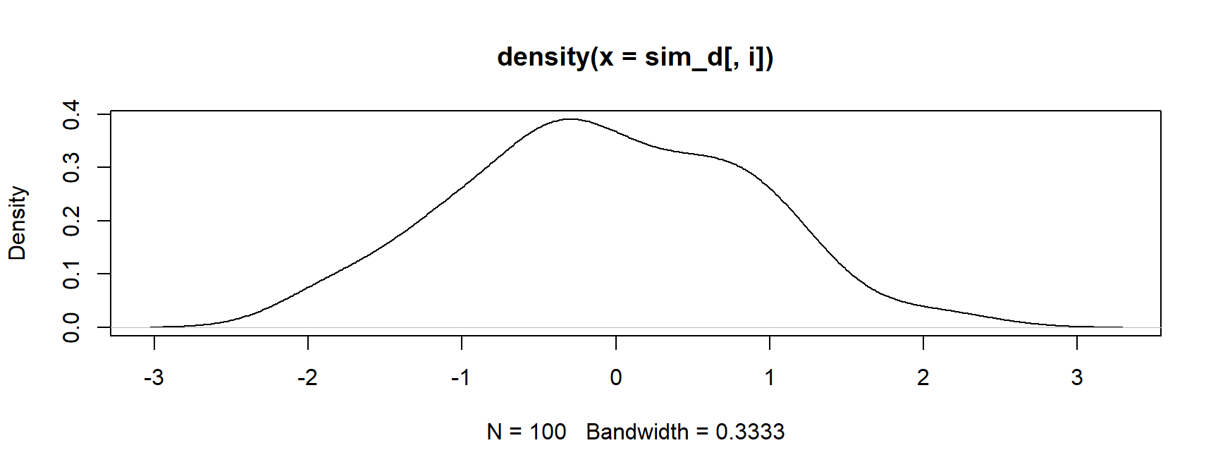
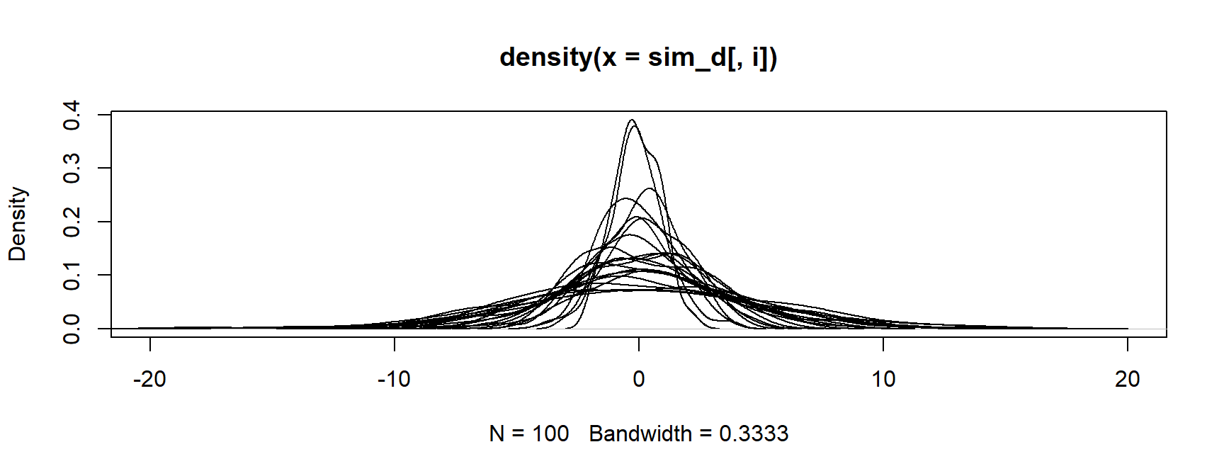
Base `R` Method

Finally, loop through all the other densities

plot(densities[[1]], xlim = c(-20, 20))

for(i in seq(2, length(densities))) {
    lines(x = densities[[i]]$x, 
          y = densities[[i]]$y) 
}

Skipping iterations

On the prior slide, I set the index to skip over the first by using seq(2, length(densities))
Alternatively, the loop could have been written like this

plot(densities[[1]], xlim = c(-20, 20))

for(i in seq_along(densities)) {
    if(i == 1) next
    lines(x = densities[[i]]$x, 
          y = densities[[i]]$y) 
}

Of course, someone has to write loops. It doesn’t have to be you.

– Jenny Bryan

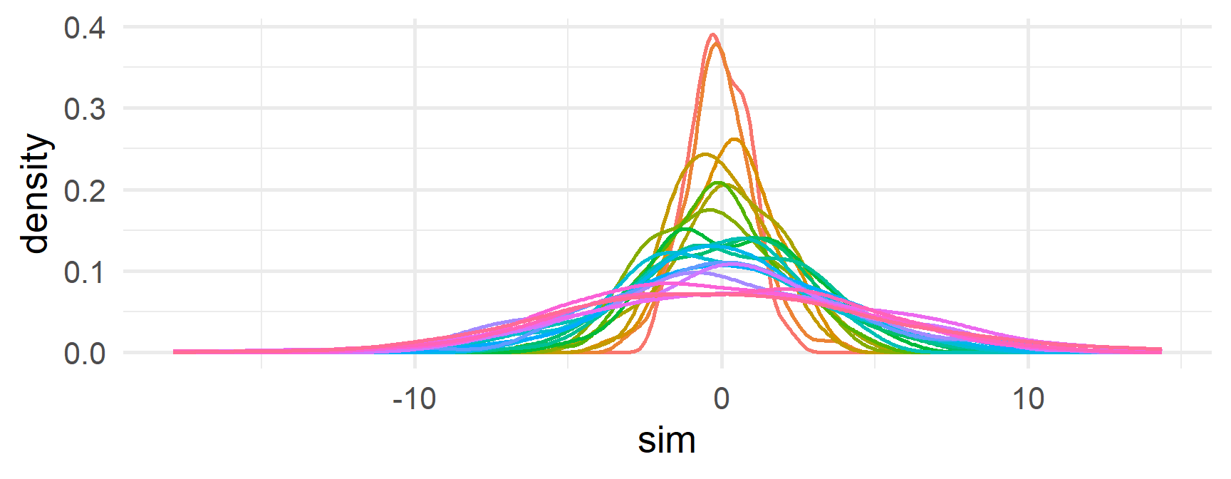
`tidyverse`

One of the best things about the tidyverse is that it often does the looping for you

pd <- sim_d |>
    pivot_longer(
      everything(),
      names_to = "sd", 
      values_to = "sim",
      names_prefix = "sd_",
      names_ptypes = list(
        sd = factor()
      )
    ) 

ggplot(pd, aes(sim)) +
 geom_density(aes(color = sd)) +
 guides(color = "none")

`break`

Stop an iteration if a condition is met with break

break on “ugli fruit”

fruit

 [1] "apple"             "apricot"           "avocado"          
 [4] "banana"            "bell pepper"       "bilberry"         
 [7] "blackberry"        "blackcurrant"      "blood orange"     
[10] "blueberry"         "boysenberry"       "breadfruit"       
[13] "canary melon"      "cantaloupe"        "cherimoya"        
[16] "cherry"            "chili pepper"      "clementine"       
[19] "cloudberry"        "coconut"           "cranberry"        
[22] "cucumber"          "currant"           "damson"           
[25] "date"              "dragonfruit"       "durian"           
[28] "eggplant"          "elderberry"        "feijoa"           
[31] "fig"               "goji berry"        "gooseberry"       
[34] "grape"             "grapefruit"        "guava"            
[37] "honeydew"          "huckleberry"       "jackfruit"        
[40] "jambul"            "jujube"            "kiwi fruit"       
[43] "kumquat"           "lemon"             "lime"             
[46] "loquat"            "lychee"            "mandarine"        
[49] "mango"             "mulberry"          "nectarine"        
[52] "nut"               "olive"             "orange"           
[55] "pamelo"            "papaya"            "passionfruit"     
[58] "peach"             "pear"              "persimmon"        
[61] "physalis"          "pineapple"         "plum"             
[64] "pomegranate"       "pomelo"            "purple mangosteen"
[67] "quince"            "raisin"            "rambutan"         
[70] "raspberry"         "redcurrant"        "rock melon"       
[73] "salal berry"       "satsuma"           "star fruit"       
[76] "strawberry"        "tamarillo"         "tangerine"        
[79] "ugli fruit"        "watermelon"

set.seed(3000)

rand_fruit <- vector("character", 100)

for(i in seq_along(rand_fruit)) {
    rand_fruit[i] <- sample(fruit, 1)
    if(any(rand_fruit == "ugli fruit")) {
        break
    }
}

rand_fruit

  [1] "cherimoya"    "lychee"       "passionfruit" "blueberry"    "cranberry"   
  [6] "currant"      "boysenberry"  "chili pepper" "avocado"      "blood orange"
 [11] "ugli fruit"   ""             ""             ""             ""            
 [16] ""             ""             ""             ""             ""            
 [21] ""             ""             ""             ""             ""            
 [26] ""             ""             ""             ""             ""            
 [31] ""             ""             ""             ""             ""            
 [36] ""             ""             ""             ""             ""            
 [41] ""             ""             ""             ""             ""            
 [46] ""             ""             ""             ""             ""            
 [51] ""             ""             ""             ""             ""            
 [56] ""             ""             ""             ""             ""            
 [61] ""             ""             ""             ""             ""            
 [66] ""             ""             ""             ""             ""            
 [71] ""             ""             ""             ""             ""            
 [76] ""             ""             ""             ""             ""            
 [81] ""             ""             ""             ""             ""            
 [86] ""             ""             ""             ""             ""            
 [91] ""             ""             ""             ""             ""            
 [96] ""             ""             ""             ""             ""

`next`

Skip an iteration without terminating the loop with next

skip “ugli fruit”

set.seed(3000)

rand_fruit <- vector("character", 100)

for(i in seq_along(rand_fruit)) {
  
  f <- sample(fruit, 1)
  
  if(f == "ugli fruit") {
    next
  }
  
  rand_fruit[i] <- f
}

sum(str_detect(rand_fruit, "ugli fruit"))

[1] 0

Last thought on `for` loops

You generally shouldn’t need to use for loops for data analysis tasks

apply() (next) and map() (next week) provide more robust solutions to most problems

*apply

`lapply()`

One of numerous functionals in R
- A functional “takes a function as an input and returns a vector as output” (AdvR, Ch. 9)
lapply() will always return a list
lapply(x, FUN, ...)

Simple examples

Loop through a data frame

Remember - a data frame is a list. We can loop through it easily

library(palmerpenguins)
lapply(penguins, is.numeric)

$species
[1] FALSE

$island
[1] FALSE

$bill_length_mm
[1] TRUE

$bill_depth_mm
[1] TRUE

$flipper_length_mm
[1] TRUE

$body_mass_g
[1] TRUE

$sex
[1] FALSE

$year
[1] TRUE

lapply(mtcars, mean)

$mpg
[1] 20.09062

$cyl
[1] 6.1875

$disp
[1] 230.7219

$hp
[1] 146.6875

$drat
[1] 3.596563

$wt
[1] 3.21725

$qsec
[1] 17.84875

$vs
[1] 0.4375

$am
[1] 0.40625

$gear
[1] 3.6875

$carb
[1] 2.8125

Revisiting our simulation with \(n = 10\)

10 cases from random normal distribution

Our for loop version

increments <- seq(1, 5, by = 0.2)

simulated <- vector("list", length(increments))

for(i in seq_along(simulated)) {
    simulated[[i]] <- rnorm(10, 0, increments[i]) 
}

simulated

[[1]]
 [1]  0.7019659  1.4080729  1.5855049 -0.1159594 -1.6184577 -0.8685868
 [7]  0.5725353  1.5020997  0.4776544  0.5704263

[[2]]
 [1] -1.5032111 -0.4635517  0.5843735  2.5511473  0.8311559 -2.5939943
 [7] -1.3946632 -0.3744163 -0.9565903 -0.3334137

[[3]]
 [1]  1.3987541  1.3138154  1.1952521 -0.7280929 -0.9774022 -2.3748910
 [7]  0.2211581  2.0439555  0.6597643  0.9247177

[[4]]
 [1] -1.17938792 -0.85090394 -1.66911850  0.60580107 -0.09319063  0.96424908
 [7] -0.71573874 -0.84862914 -2.84366893  2.74051043

[[5]]
 [1] -1.67473502  3.78627668  2.21760469  1.79871989  0.61076082  2.26739975
 [7]  0.40318730 -1.47898063 -0.93028381 -0.06112215

[[6]]
 [1] -0.39360342  2.63045923  0.13683130 -0.30129628 -2.80950121 -0.45100320
 [7]  1.85287700  0.08379172 -3.35182610 -1.13943533

[[7]]
 [1] -0.8792638 -0.2015623  0.8712158 -4.0155096  1.4829769 -1.2439822
 [7] -4.9190550  1.9448742  0.6006172 -3.1500311

[[8]]
 [1] -1.19258914  1.70128147 -1.01709724  4.12107298  0.39844070 -0.03773795
 [7] -0.88892905  1.72924626 -2.20431086  3.55655316

[[9]]
 [1] -0.8109234  2.2415188 -4.3428035 -1.3887998  0.9478032 -2.1510850
 [7]  2.2464380  2.1790652  0.2658378 -0.5050961

[[10]]
 [1] -3.8380453  1.8707884 -4.7180945 -5.2706985  0.7637031 -2.5150921
 [7]  0.1398676  4.7475136  1.8262695  0.8878070

[[11]]
 [1] -0.7124232  5.6971345  0.4168275  2.1707873  0.4078937  0.8236137
 [7]  0.4166894 -1.1700535  0.2813558 -1.7013374

[[12]]
 [1]  3.6684601 -6.4950553  2.7195886 -4.0825655 -1.3228556  0.3686458
 [7] -1.7199430  4.0405103  1.8186114  2.6708650

[[13]]
 [1]  3.4796287 -4.7070236  6.3598681 -0.2484373  3.3232871  1.8303518
 [7] -6.6345432 -2.6541128  4.3034350 -6.2735923

[[14]]
 [1]  0.9638453 -2.2051130 -0.2938058 -0.1776934 -0.2382037 -2.5918608
 [7]  8.2087316  6.3124395 -1.6617223 -5.0983245

[[15]]
 [1] -3.356816 -9.866520  1.270889 -5.050831  4.819798 -4.276553 -5.123649
 [8]  4.800624  2.900262  4.638832

[[16]]
 [1]  1.2533397 -0.7967168 -3.4747042  0.7045451  2.6577155 -1.1389303
 [7] -0.9931517 -0.6158335  3.1899898 -2.0015935

[[17]]
 [1] -2.5475101  1.9713666  1.7382913  0.1806804 -2.3263909  3.2468837
 [7] -2.3498898 -0.4262246 -9.2894332  2.9332861

[[18]]
 [1]  7.2226066  4.2077777 -1.9218792  0.1525742 -2.4302173  7.5949019
 [7]  1.4443248 -3.0579550 -4.6065755 -2.4429780

[[19]]
 [1]  3.006982  2.402910 -4.455305 -1.365753  1.007137  1.945525  5.731369
 [8]  2.643082  7.253715 -1.310914

[[20]]
 [1] -4.84015782  1.13853303 -1.26893048  0.03200417 -1.08084880  1.57557106
 [7]  0.37274324  1.74783587  3.75306613 -0.24459380

[[21]]
 [1]  7.1202227 -5.5543948  1.4972206  4.8239050 -1.9867446  0.7982388
 [7] -0.8702481 -4.7798742 -2.4762099  6.6618692

The `lapply` version

increments <- seq(1, 5, by = 0.2)
sim_l <- lapply(increments, function(sd) rnorm(10, 0, sd))
sim_l

[[1]]
 [1] -0.492977465 -1.326315004 -1.277971738 -1.786735667 -0.029929162
 [6]  0.821401221 -1.901137076 -0.313659636  0.007199708 -0.940656172

[[2]]
 [1]  0.02293225  0.27576005  0.98030384  1.48113369 -1.87152339 -0.28627466
 [7]  1.51132454  1.56102968 -0.02240571 -2.80846340

[[3]]
 [1]  1.4057812  1.1853134 -1.2570415  0.6509708 -0.6405013  0.6936492
 [7] -1.9660866  1.7420709 -1.4611224  0.1316577

[[4]]
 [1]  0.7812576 -2.9256970 -1.5436066 -2.5333862  0.6171761  0.7044896
 [7] -0.4006856 -0.6106846 -0.1082784  0.7174894

[[5]]
 [1]  1.5374167  0.2505228 -1.2636145 -0.9425670 -2.3026569  1.8802193
 [7]  1.4040287 -0.5680369 -1.7274334  0.6360815

[[6]]
 [1] -2.0901501 -0.5947297  1.3656397  0.9351094 -3.3431900 -4.0962263
 [7] -2.0610299  0.7385466 -2.3327358  0.2866699

[[7]]
 [1]  3.2682871 -0.3279264  1.4030807  0.1635299 -2.8962721 -2.9090211
 [7] -1.1082169  3.1683640  1.0964915 -4.1445029

[[8]]
 [1]  1.0202599 -2.1033574  3.0265243  0.4845599 -1.0732037 -1.6051391
 [7] -4.5692419  1.3335215 -1.1335379  0.8800409

[[9]]
 [1] -0.4299886  2.3957394 -1.1279263  3.1767972 -2.1287808  1.1345961
 [7]  1.6635893  1.0742162  3.9675515 -3.4037107

[[10]]
 [1]  3.90943708 -0.47550222 -0.05090254 -3.79433049  2.16843003  0.49479999
 [7]  1.95194176  1.10057432  1.36113548 -1.63364698

[[11]]
 [1]  3.5635989 -3.0480015 -1.9094632 -1.9366025  8.0425229 -2.2570386
 [7]  2.0810249  0.9133481  1.6115470 -2.6532489

[[12]]
 [1]  2.0564643  1.6226583 -3.5424946 -1.2795244  3.0515716 -2.8734308
 [7] -6.7897219 -4.8821254  0.3650476  0.8821632

[[13]]
 [1]  1.9075504 -4.5077636  3.9142408 -5.9789372 -0.6233262 -4.4681065
 [7]  6.1586895 -0.5944915 -5.7116492  6.2312506

[[14]]
 [1] -9.0647986  7.0709317 -0.7426188 -4.1666946  4.2353914  6.2356319
 [7] -4.8357753 -2.9394862  0.8712302 -2.6338505

[[15]]
 [1] -0.03001855 -1.02837565  3.37147544 -5.63001035 -0.17605241 -1.07074739
 [7]  0.89752455  2.51672975  7.04064931  5.80698376

[[16]]
 [1]  4.0908012 -6.9555688 -0.3289718  1.4108902 -8.8010982  3.8916145
 [7] -0.9847857  2.7977282 -6.0947913 -6.1222646

[[17]]
 [1] -3.9260707  1.9920454  9.1815418 -0.6280606 -6.0461562 -0.7289214
 [7] -6.7850840 -6.2090067  1.0525724 -1.4549614

[[18]]
 [1] -0.55385742  0.16206180  4.73568372 -1.58979352 -2.31641650 -5.44034366
 [7] -0.51173292 -2.19302330  3.52421093 -0.07061819

[[19]]
 [1]   1.947770 -10.807521  -1.124952  -7.733490  -3.695339 -10.566181
 [7]  -2.359878  -3.132563   0.843549   1.468815

[[20]]
 [1] -8.0996104  2.0494324  4.7118897 -0.7059947  0.8819594  7.7818183
 [7]  5.7361528 -2.1250988  2.4668712 -4.9415075

[[21]]
 [1]  1.9603391 -7.3245899  1.7117409 -2.2333932  3.9712935 -5.0422957
 [7]  0.9769575 -1.9214953  1.4732655  2.7652785

Back to this one

lapply(penguins, is.numeric)

$species
[1] FALSE

$island
[1] FALSE

$bill_length_mm
[1] TRUE

$bill_depth_mm
[1] TRUE

$flipper_length_mm
[1] TRUE

$body_mass_g
[1] TRUE

$sex
[1] FALSE

$year
[1] TRUE

Add a condition

lapply(penguins, function(x) {
    if(is.numeric(x)) {
        mean(x, na.rm = TRUE)
    }
})

$species
NULL

$island
NULL

$bill_length_mm
[1] 43.92193

$bill_depth_mm
[1] 17.15117

$flipper_length_mm
[1] 200.9152

$body_mass_g
[1] 4201.754

$sex
NULL

$year
[1] 2008.029

Add a second condition

lapply(penguins, function(x) {
    if(is.numeric(x)) {
      return(mean(x, na.rm = TRUE))
    }
    else if(is.character(x) | is.factor(x)) {
      return(table(x))
  }
})

$species
x
   Adelie Chinstrap    Gentoo 
      152        68       124 

$island
x
   Biscoe     Dream Torgersen 
      168       124        52 

$bill_length_mm
[1] 43.92193

$bill_depth_mm
[1] 17.15117

$flipper_length_mm
[1] 200.9152

$body_mass_g
[1] 4201.754

$sex
x
female   male 
   165    168 

$year
[1] 2008.029

Passing arguments

There’s missing data, so this won’t work

head(airquality)

  Ozone Solar.R Wind Temp Month Day
1    41     190  7.4   67     5   1
2    36     118  8.0   72     5   2
3    12     149 12.6   74     5   3
4    18     313 11.5   62     5   4
5    NA      NA 14.3   56     5   5
6    28      NA 14.9   66     5   6

lapply(airquality, mean)

$Ozone
[1] NA

$Solar.R
[1] NA

$Wind
[1] 9.957516

$Temp
[1] 77.88235

$Month
[1] 6.993464

$Day
[1] 15.80392

But this will

lapply(airquality, mean, na.rm = TRUE)

$Ozone
[1] 42.12931

$Solar.R
[1] 185.9315

$Wind
[1] 9.957516

$Temp
[1] 77.88235

$Month
[1] 6.993464

$Day
[1] 15.80392

Alternative notation

The prior code could also be written like this

lapply(airquality, function(x) mean(x, na.rm = TRUE))

$Ozone
[1] 42.12931

$Solar.R
[1] 185.9315

$Wind
[1] 9.957516

$Temp
[1] 77.88235

$Month
[1] 6.993464

$Day
[1] 15.80392

My brain likes this better

Alternative notation

This will NOT work

lapply(airquality, mean(x, na.rm = TRUE))

Error in `match.fun()`:
! 'mean(x, na.rm = TRUE)' is not a function, character or symbol

This WILL

lapply(airquality, mean, na.rm = TRUE)

$Ozone
[1] 42.12931

$Solar.R
[1] 185.9315

$Wind
[1] 9.957516

$Temp
[1] 77.88235

$Month
[1] 6.993464

$Day
[1] 15.80392

Simulation again

set.seed(3000)
lapply(seq(1, 5, 0.2), rnorm, n = 10, mean = 0)

[[1]]
 [1]  1.2582925  0.6447519  0.4633460  0.7703058 -0.2263347 -0.3515479
 [7] -0.6493198 -1.2625922 -1.6971350 -1.8340239

[[2]]
 [1] -0.98745656 -1.94162010  0.36621285  1.79180419  0.03449261 -0.67549407
 [7]  0.54284453  0.72178563  1.32617338 -2.34937275

[[3]]
 [1] -0.06812657  1.38810114 -0.91551411 -0.64826439 -1.44302498 -1.02579387
 [7]  0.80129321 -0.78811938 -1.76193450 -0.88391729

[[4]]
 [1] -0.5450989  0.7175976  1.5508069 -1.3445723  1.6618678 -0.0495352
 [7] -0.5573398 -0.1277775 -3.5923124  1.2796936

[[5]]
 [1] -4.4550368  2.3194451  0.8959171  2.5835431 -1.1888322 -1.8311366
 [7] -0.3824221 -1.1450434  0.5915765 -1.4560164

[[6]]
 [1]  1.4773287 -0.3317452  0.1027664  0.3976797  0.3269631 -0.2564408
 [7]  5.2480829  3.9702687  3.3295696 -2.0356887

[[7]]
 [1] -1.6995589 -1.2256900  3.5602090 -0.2417684 -0.5324828  1.8777524
 [7] -2.0724353 -2.8530262 -1.1922938  0.1842753

[[8]]
 [1] -1.3341336 -2.6062520 -2.7785042 -0.5129759  4.2123126  1.3930112
 [7]  5.6435182  1.4840936 -0.5187353  0.6345386

[[9]]
 [1]  0.7767619 -3.2902109 -3.3817425  0.6591373  0.6431185 -0.8448418
 [7]  1.8194023  3.1956026  3.8377482  4.6509330

[[10]]
 [1] -2.7682851  0.7743240 -2.5806469 -0.2963955 -0.5855121 -0.2799172
 [7] -2.8184065 -0.9122830  0.9552384 -2.8058944

[[11]]
 [1] -1.2638710  1.9250688  3.0155007 -0.9679650 -1.6901458  0.9453726
 [7] -6.3824047  1.6183184 -2.5262227 -2.5155382

[[12]]
 [1] -0.8360622  4.6567564 -1.9687763  2.1833804  0.1476822 -2.2601583
 [7] -0.7957750 -3.0078040  4.1782934 -0.6554053

[[13]]
 [1] -4.42386931 -2.46107097  1.97132477  2.50801791  5.79837506  6.32623541
 [7] -4.06609414 -0.06348689  2.34150869  3.14411805

[[14]]
 [1]  5.2020713  5.9590067  1.6950772 -6.7035571  1.5852297 -3.2095910
 [7]  4.9312293 -2.5348971 -7.0058786  0.7334374

[[15]]
 [1] -3.3942288  1.4462102 -1.5728799 -0.2756218 -0.1576324  2.4748973
 [7]  1.5381645 -2.1900007  2.4551050  7.9625057

[[16]]
 [1]  5.117237 -2.849735 13.196387 -3.702533 -2.779757 -2.019801 -2.463081
 [8] -2.521757 -1.058628  2.298301

[[17]]
 [1]  5.32913199 -1.33174468  0.09956103 -3.43446361  4.92644150 -3.15962941
 [7] -1.92752643 -5.05937551  1.69674715  3.38437133

[[18]]
 [1]  1.4065749 -1.1391737 -5.9956124 -0.2993126 -2.6370933  0.2733555
 [7]  1.3994970 -6.0855343  1.9985985 -6.1843592

[[19]]
 [1]  2.930842  5.686328  5.595754 -7.956035 -4.132702 -4.313917 -5.387319
 [8]  1.501185 -8.421652  2.561221

[[20]]
 [1]  1.1546085 -1.8250863 -0.6488753 -4.2618750 -0.1084859 -3.1701360
 [7] -1.5113640 -2.2808379  1.4172582  2.6221386

[[21]]
 [1]   5.035385   4.713422  10.053528  -3.848520   4.548012 -11.439839
 [7]   3.202310   5.052674  -2.349106  11.366291

Equivalent to

set.seed(3000)
lapply(seq(1, 5, by = 0.2), function(sd) rnorm(10, 0, sd))

[[1]]
 [1]  1.2582925  0.6447519  0.4633460  0.7703058 -0.2263347 -0.3515479
 [7] -0.6493198 -1.2625922 -1.6971350 -1.8340239

[[2]]
 [1] -0.98745656 -1.94162010  0.36621285  1.79180419  0.03449261 -0.67549407
 [7]  0.54284453  0.72178563  1.32617338 -2.34937275

[[3]]
 [1] -0.06812657  1.38810114 -0.91551411 -0.64826439 -1.44302498 -1.02579387
 [7]  0.80129321 -0.78811938 -1.76193450 -0.88391729

[[4]]
 [1] -0.5450989  0.7175976  1.5508069 -1.3445723  1.6618678 -0.0495352
 [7] -0.5573398 -0.1277775 -3.5923124  1.2796936

[[5]]
 [1] -4.4550368  2.3194451  0.8959171  2.5835431 -1.1888322 -1.8311366
 [7] -0.3824221 -1.1450434  0.5915765 -1.4560164

[[6]]
 [1]  1.4773287 -0.3317452  0.1027664  0.3976797  0.3269631 -0.2564408
 [7]  5.2480829  3.9702687  3.3295696 -2.0356887

[[7]]
 [1] -1.6995589 -1.2256900  3.5602090 -0.2417684 -0.5324828  1.8777524
 [7] -2.0724353 -2.8530262 -1.1922938  0.1842753

[[8]]
 [1] -1.3341336 -2.6062520 -2.7785042 -0.5129759  4.2123126  1.3930112
 [7]  5.6435182  1.4840936 -0.5187353  0.6345386

[[9]]
 [1]  0.7767619 -3.2902109 -3.3817425  0.6591373  0.6431185 -0.8448418
 [7]  1.8194023  3.1956026  3.8377482  4.6509330

[[10]]
 [1] -2.7682851  0.7743240 -2.5806469 -0.2963955 -0.5855121 -0.2799172
 [7] -2.8184065 -0.9122830  0.9552384 -2.8058944

[[11]]
 [1] -1.2638710  1.9250688  3.0155007 -0.9679650 -1.6901458  0.9453726
 [7] -6.3824047  1.6183184 -2.5262227 -2.5155382

[[12]]
 [1] -0.8360622  4.6567564 -1.9687763  2.1833804  0.1476822 -2.2601583
 [7] -0.7957750 -3.0078040  4.1782934 -0.6554053

[[13]]
 [1] -4.42386931 -2.46107097  1.97132477  2.50801791  5.79837506  6.32623541
 [7] -4.06609414 -0.06348689  2.34150869  3.14411805

[[14]]
 [1]  5.2020713  5.9590067  1.6950772 -6.7035571  1.5852297 -3.2095910
 [7]  4.9312293 -2.5348971 -7.0058786  0.7334374

[[15]]
 [1] -3.3942288  1.4462102 -1.5728799 -0.2756218 -0.1576324  2.4748973
 [7]  1.5381645 -2.1900007  2.4551050  7.9625057

[[16]]
 [1]  5.117237 -2.849735 13.196387 -3.702533 -2.779757 -2.019801 -2.463081
 [8] -2.521757 -1.058628  2.298301

[[17]]
 [1]  5.32913199 -1.33174468  0.09956103 -3.43446361  4.92644150 -3.15962941
 [7] -1.92752643 -5.05937551  1.69674715  3.38437133

[[18]]
 [1]  1.4065749 -1.1391737 -5.9956124 -0.2993126 -2.6370933  0.2733555
 [7]  1.3994970 -6.0855343  1.9985985 -6.1843592

[[19]]
 [1]  2.930842  5.686328  5.595754 -7.956035 -4.132702 -4.313917 -5.387319
 [8]  1.501185 -8.421652  2.561221

[[20]]
 [1]  1.1546085 -1.8250863 -0.6488753 -4.2618750 -0.1084859 -3.1701360
 [7] -1.5113640 -2.2808379  1.4172582  2.6221386

[[21]]
 [1]   5.035385   4.713422  10.053528  -3.848520   4.548012 -11.439839
 [7]   3.202310   5.052674  -2.349106  11.366291

Operations by group

Mimic `dplyr::group_by()`

with split()

by_cyl <- split(mtcars, mtcars$cyl)
by_cyl

$`4`
                mpg cyl  disp  hp drat    wt  qsec vs am gear carb
Datsun 710     22.8   4 108.0  93 3.85 2.320 18.61  1  1    4    1
Merc 240D      24.4   4 146.7  62 3.69 3.190 20.00  1  0    4    2
Merc 230       22.8   4 140.8  95 3.92 3.150 22.90  1  0    4    2
Fiat 128       32.4   4  78.7  66 4.08 2.200 19.47  1  1    4    1
Honda Civic    30.4   4  75.7  52 4.93 1.615 18.52  1  1    4    2
Toyota Corolla 33.9   4  71.1  65 4.22 1.835 19.90  1  1    4    1
Toyota Corona  21.5   4 120.1  97 3.70 2.465 20.01  1  0    3    1
Fiat X1-9      27.3   4  79.0  66 4.08 1.935 18.90  1  1    4    1
Porsche 914-2  26.0   4 120.3  91 4.43 2.140 16.70  0  1    5    2
Lotus Europa   30.4   4  95.1 113 3.77 1.513 16.90  1  1    5    2
Volvo 142E     21.4   4 121.0 109 4.11 2.780 18.60  1  1    4    2

$`6`
                mpg cyl  disp  hp drat    wt  qsec vs am gear carb
Mazda RX4      21.0   6 160.0 110 3.90 2.620 16.46  0  1    4    4
Mazda RX4 Wag  21.0   6 160.0 110 3.90 2.875 17.02  0  1    4    4
Hornet 4 Drive 21.4   6 258.0 110 3.08 3.215 19.44  1  0    3    1
Valiant        18.1   6 225.0 105 2.76 3.460 20.22  1  0    3    1
Merc 280       19.2   6 167.6 123 3.92 3.440 18.30  1  0    4    4
Merc 280C      17.8   6 167.6 123 3.92 3.440 18.90  1  0    4    4
Ferrari Dino   19.7   6 145.0 175 3.62 2.770 15.50  0  1    5    6

$`8`
                     mpg cyl  disp  hp drat    wt  qsec vs am gear carb
Hornet Sportabout   18.7   8 360.0 175 3.15 3.440 17.02  0  0    3    2
Duster 360          14.3   8 360.0 245 3.21 3.570 15.84  0  0    3    4
Merc 450SE          16.4   8 275.8 180 3.07 4.070 17.40  0  0    3    3
Merc 450SL          17.3   8 275.8 180 3.07 3.730 17.60  0  0    3    3
Merc 450SLC         15.2   8 275.8 180 3.07 3.780 18.00  0  0    3    3
Cadillac Fleetwood  10.4   8 472.0 205 2.93 5.250 17.98  0  0    3    4
Lincoln Continental 10.4   8 460.0 215 3.00 5.424 17.82  0  0    3    4
Chrysler Imperial   14.7   8 440.0 230 3.23 5.345 17.42  0  0    3    4
Dodge Challenger    15.5   8 318.0 150 2.76 3.520 16.87  0  0    3    2
AMC Javelin         15.2   8 304.0 150 3.15 3.435 17.30  0  0    3    2
Camaro Z28          13.3   8 350.0 245 3.73 3.840 15.41  0  0    3    4
Pontiac Firebird    19.2   8 400.0 175 3.08 3.845 17.05  0  0    3    2
Ford Pantera L      15.8   8 351.0 264 4.22 3.170 14.50  0  1    5    4
Maserati Bora       15.0   8 301.0 335 3.54 3.570 14.60  0  1    5    8

Mimic `dplyr::group_by()`

str(by_cyl)

List of 3
 $ 4:'data.frame':  11 obs. of  11 variables:
  ..$ mpg : num [1:11] 22.8 24.4 22.8 32.4 30.4 33.9 21.5 27.3 26 30.4 ...
  ..$ cyl : num [1:11] 4 4 4 4 4 4 4 4 4 4 ...
  ..$ disp: num [1:11] 108 146.7 140.8 78.7 75.7 ...
  ..$ hp  : num [1:11] 93 62 95 66 52 65 97 66 91 113 ...
  ..$ drat: num [1:11] 3.85 3.69 3.92 4.08 4.93 4.22 3.7 4.08 4.43 3.77 ...
  ..$ wt  : num [1:11] 2.32 3.19 3.15 2.2 1.61 ...
  ..$ qsec: num [1:11] 18.6 20 22.9 19.5 18.5 ...
  ..$ vs  : num [1:11] 1 1 1 1 1 1 1 1 0 1 ...
  ..$ am  : num [1:11] 1 0 0 1 1 1 0 1 1 1 ...
  ..$ gear: num [1:11] 4 4 4 4 4 4 3 4 5 5 ...
  ..$ carb: num [1:11] 1 2 2 1 2 1 1 1 2 2 ...
 $ 6:'data.frame':  7 obs. of  11 variables:
  ..$ mpg : num [1:7] 21 21 21.4 18.1 19.2 17.8 19.7
  ..$ cyl : num [1:7] 6 6 6 6 6 6 6
  ..$ disp: num [1:7] 160 160 258 225 168 ...
  ..$ hp  : num [1:7] 110 110 110 105 123 123 175
  ..$ drat: num [1:7] 3.9 3.9 3.08 2.76 3.92 3.92 3.62
  ..$ wt  : num [1:7] 2.62 2.88 3.21 3.46 3.44 ...
  ..$ qsec: num [1:7] 16.5 17 19.4 20.2 18.3 ...
  ..$ vs  : num [1:7] 0 0 1 1 1 1 0
  ..$ am  : num [1:7] 1 1 0 0 0 0 1
  ..$ gear: num [1:7] 4 4 3 3 4 4 5
  ..$ carb: num [1:7] 4 4 1 1 4 4 6
 $ 8:'data.frame':  14 obs. of  11 variables:
  ..$ mpg : num [1:14] 18.7 14.3 16.4 17.3 15.2 10.4 10.4 14.7 15.5 15.2 ...
  ..$ cyl : num [1:14] 8 8 8 8 8 8 8 8 8 8 ...
  ..$ disp: num [1:14] 360 360 276 276 276 ...
  ..$ hp  : num [1:14] 175 245 180 180 180 205 215 230 150 150 ...
  ..$ drat: num [1:14] 3.15 3.21 3.07 3.07 3.07 2.93 3 3.23 2.76 3.15 ...
  ..$ wt  : num [1:14] 3.44 3.57 4.07 3.73 3.78 ...
  ..$ qsec: num [1:14] 17 15.8 17.4 17.6 18 ...
  ..$ vs  : num [1:14] 0 0 0 0 0 0 0 0 0 0 ...
  ..$ am  : num [1:14] 0 0 0 0 0 0 0 0 0 0 ...
  ..$ gear: num [1:14] 3 3 3 3 3 3 3 3 3 3 ...
  ..$ carb: num [1:14] 2 4 3 3 3 4 4 4 2 2 ...

Mimic `dplyr::group_by()`

lapply(by_cyl, function(x) mean(x$mpg))

$`4`
[1] 26.66364

$`6`
[1] 19.74286

$`8`
[1] 15.1

lapply(by_cyl, function(x) mean(x[["mpg"]]))

$`4`
[1] 26.66364

$`6`
[1] 19.74286

$`8`
[1] 15.1

Or even (less ideal)

lapply(by_cyl, function(x) mean(x[[1]]))

$`4`
[1] 26.66364

$`6`
[1] 19.74286

$`8`
[1] 15.1

Because we are just subsettting the list

Your turn

Try splitting the penguins dataset by species and calculating the average bill_length_mm

demo

Solution

peng_split <- split(penguins, penguins$species)

lapply(peng_split, function(x) mean(x$bill_length_mm, na.rm = TRUE))

$Adelie
[1] 38.79139

$Chinstrap
[1] 48.83382

$Gentoo
[1] 47.50488

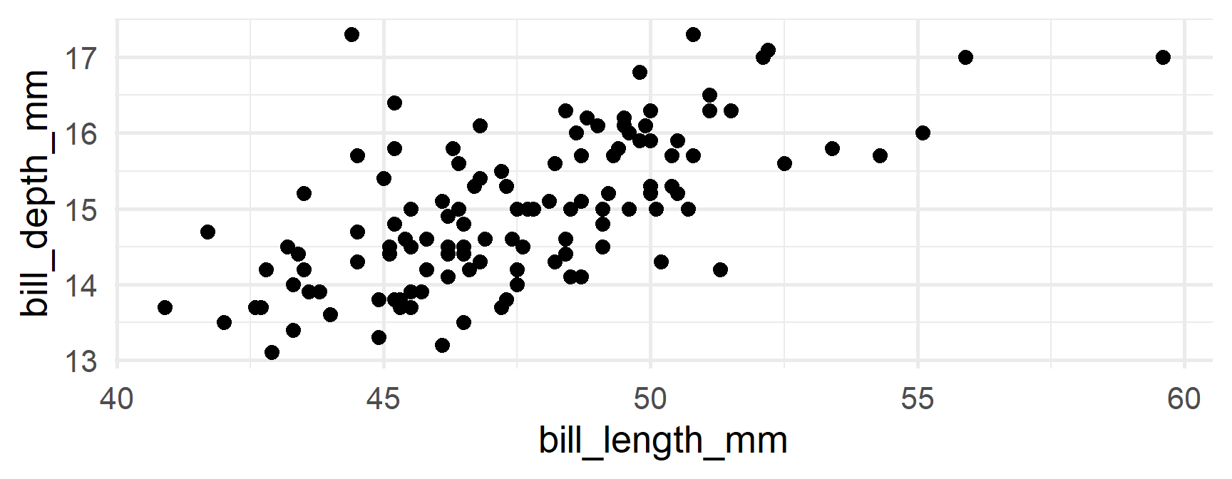
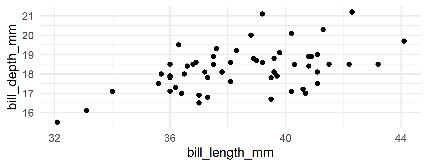
Produce separate plots

lapply(by_cyl, function(x) {
    ggplot(x, aes(disp, mpg)) +
        geom_point() +
        geom_smooth()
})

$`4`


$`6`


$`8`

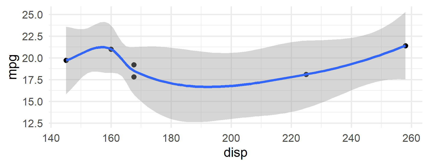
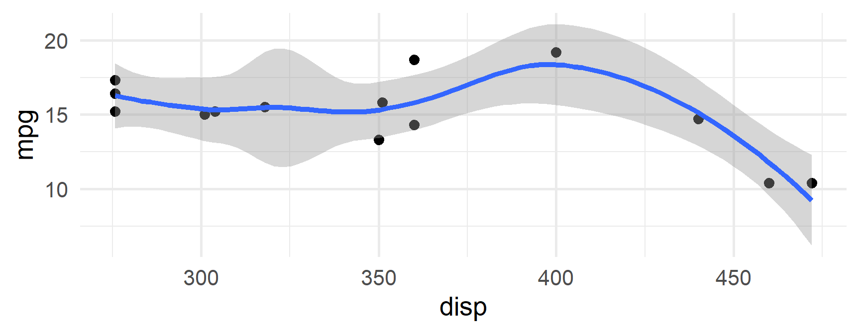
Your turn

Produce separate plots of the relation between bill_length_mm and body_mass_g

share code

Saving

You can extend this example further by saving the plot outputs to an object, then looping through that object to save the plots to disk
Using functionals, this would require parallel iterations, which we’ll cover later (need to loop through plots and a file name)
Could extend it fairly easily with a for loop

Saving with `for` loop

Save plots to an object (list)

plots <- lapply(by_cyl, function(x) {
    ggplot(x, aes(disp, mpg)) +
        geom_point() +
        geom_smooth()
})

Specify file names/directory

#dir.create(here::here("plots")) 
filenames <- here::here(
  "plots",
  paste0("cyl-", names(by_cyl), ".png")
)
filenames

[1] "C:/Users/jnese/Desktop/BRT/Teaching/3_Functional-Programming/functional-programming_spring-2026/plots/cyl-4.png"
[2] "C:/Users/jnese/Desktop/BRT/Teaching/3_Functional-Programming/functional-programming_spring-2026/plots/cyl-6.png"
[3] "C:/Users/jnese/Desktop/BRT/Teaching/3_Functional-Programming/functional-programming_spring-2026/plots/cyl-8.png"

Saving

for(i in seq_along(plots)) {
    ggsave(filenames[i], # single bracket
           plots[[i]], # double bracket
           device = "png",
           width = 6.5, 
           height = 8)
}

You try!

With peng_split

More than one group

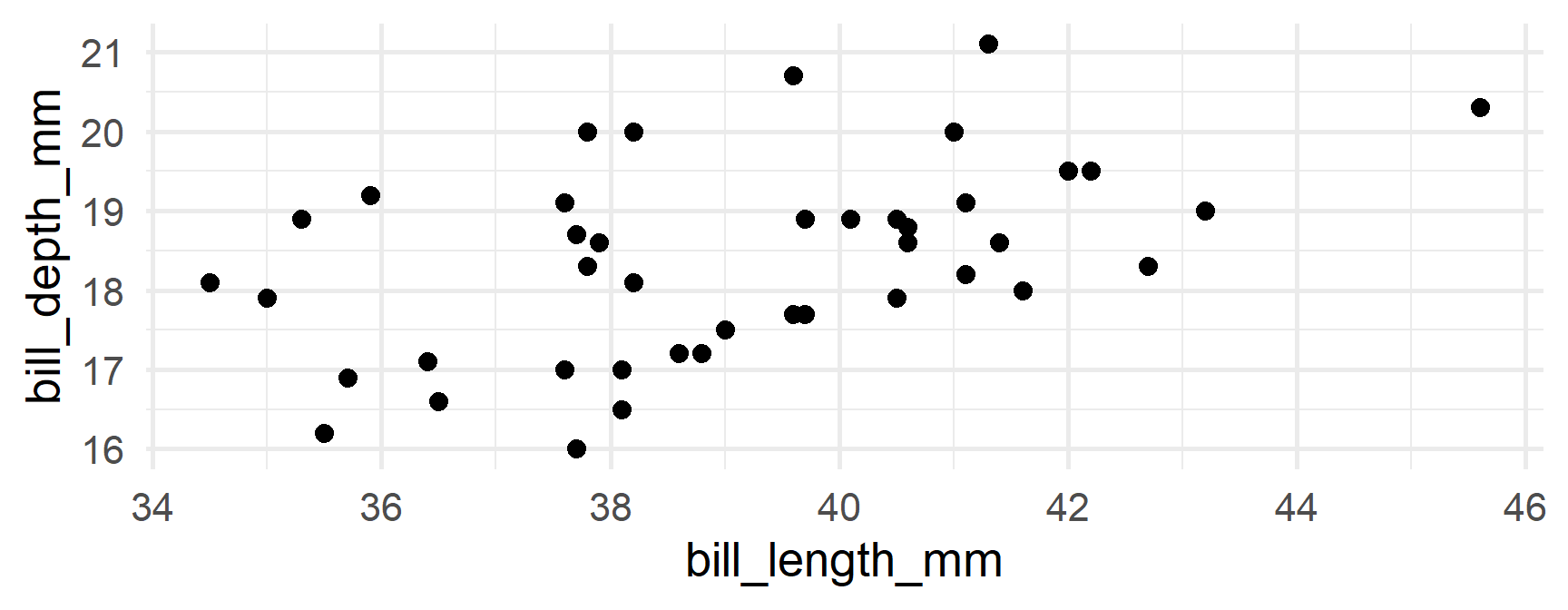
Let’s say we wanted to create a plot of bill length vs bill depth by for each combination of species/island

Just split by both!

Pass both variables as a list()

splt2 <- split(
  penguins, 
  list(penguins$species, penguins$island)
)

Inspect it

splt2

$Adelie.Biscoe
# A tibble: 44 × 8
   species island bill_length_mm bill_depth_mm flipper_length_mm body_mass_g
   <fct>   <fct>           <dbl>         <dbl>             <int>       <int>
 1 Adelie  Biscoe           37.8          18.3               174        3400
 2 Adelie  Biscoe           37.7          18.7               180        3600
 3 Adelie  Biscoe           35.9          19.2               189        3800
 4 Adelie  Biscoe           38.2          18.1               185        3950
 5 Adelie  Biscoe           38.8          17.2               180        3800
 6 Adelie  Biscoe           35.3          18.9               187        3800
 7 Adelie  Biscoe           40.6          18.6               183        3550
 8 Adelie  Biscoe           40.5          17.9               187        3200
 9 Adelie  Biscoe           37.9          18.6               172        3150
10 Adelie  Biscoe           40.5          18.9               180        3950
# ℹ 34 more rows
# ℹ 2 more variables: sex <fct>, year <int>

$Chinstrap.Biscoe
# A tibble: 0 × 8
# ℹ 8 variables: species <fct>, island <fct>, bill_length_mm <dbl>,
#   bill_depth_mm <dbl>, flipper_length_mm <int>, body_mass_g <int>, sex <fct>,
#   year <int>

$Gentoo.Biscoe
# A tibble: 124 × 8
   species island bill_length_mm bill_depth_mm flipper_length_mm body_mass_g
   <fct>   <fct>           <dbl>         <dbl>             <int>       <int>
 1 Gentoo  Biscoe           46.1          13.2               211        4500
 2 Gentoo  Biscoe           50            16.3               230        5700
 3 Gentoo  Biscoe           48.7          14.1               210        4450
 4 Gentoo  Biscoe           50            15.2               218        5700
 5 Gentoo  Biscoe           47.6          14.5               215        5400
 6 Gentoo  Biscoe           46.5          13.5               210        4550
 7 Gentoo  Biscoe           45.4          14.6               211        4800
 8 Gentoo  Biscoe           46.7          15.3               219        5200
 9 Gentoo  Biscoe           43.3          13.4               209        4400
10 Gentoo  Biscoe           46.8          15.4               215        5150
# ℹ 114 more rows
# ℹ 2 more variables: sex <fct>, year <int>

$Adelie.Dream
# A tibble: 56 × 8
   species island bill_length_mm bill_depth_mm flipper_length_mm body_mass_g
   <fct>   <fct>           <dbl>         <dbl>             <int>       <int>
 1 Adelie  Dream            39.5          16.7               178        3250
 2 Adelie  Dream            37.2          18.1               178        3900
 3 Adelie  Dream            39.5          17.8               188        3300
 4 Adelie  Dream            40.9          18.9               184        3900
 5 Adelie  Dream            36.4          17                 195        3325
 6 Adelie  Dream            39.2          21.1               196        4150
 7 Adelie  Dream            38.8          20                 190        3950
 8 Adelie  Dream            42.2          18.5               180        3550
 9 Adelie  Dream            37.6          19.3               181        3300
10 Adelie  Dream            39.8          19.1               184        4650
# ℹ 46 more rows
# ℹ 2 more variables: sex <fct>, year <int>

$Chinstrap.Dream
# A tibble: 68 × 8
   species   island bill_length_mm bill_depth_mm flipper_length_mm body_mass_g
   <fct>     <fct>           <dbl>         <dbl>             <int>       <int>
 1 Chinstrap Dream            46.5          17.9               192        3500
 2 Chinstrap Dream            50            19.5               196        3900
 3 Chinstrap Dream            51.3          19.2               193        3650
 4 Chinstrap Dream            45.4          18.7               188        3525
 5 Chinstrap Dream            52.7          19.8               197        3725
 6 Chinstrap Dream            45.2          17.8               198        3950
 7 Chinstrap Dream            46.1          18.2               178        3250
 8 Chinstrap Dream            51.3          18.2               197        3750
 9 Chinstrap Dream            46            18.9               195        4150
10 Chinstrap Dream            51.3          19.9               198        3700
# ℹ 58 more rows
# ℹ 2 more variables: sex <fct>, year <int>

$Gentoo.Dream
# A tibble: 0 × 8
# ℹ 8 variables: species <fct>, island <fct>, bill_length_mm <dbl>,
#   bill_depth_mm <dbl>, flipper_length_mm <int>, body_mass_g <int>, sex <fct>,
#   year <int>

$Adelie.Torgersen
# A tibble: 52 × 8
   species island    bill_length_mm bill_depth_mm flipper_length_mm body_mass_g
   <fct>   <fct>              <dbl>         <dbl>             <int>       <int>
 1 Adelie  Torgersen           39.1          18.7               181        3750
 2 Adelie  Torgersen           39.5          17.4               186        3800
 3 Adelie  Torgersen           40.3          18                 195        3250
 4 Adelie  Torgersen           NA            NA                  NA          NA
 5 Adelie  Torgersen           36.7          19.3               193        3450
 6 Adelie  Torgersen           39.3          20.6               190        3650
 7 Adelie  Torgersen           38.9          17.8               181        3625
 8 Adelie  Torgersen           39.2          19.6               195        4675
 9 Adelie  Torgersen           34.1          18.1               193        3475
10 Adelie  Torgersen           42            20.2               190        4250
# ℹ 42 more rows
# ℹ 2 more variables: sex <fct>, year <int>

$Chinstrap.Torgersen
# A tibble: 0 × 8
# ℹ 8 variables: species <fct>, island <fct>, bill_length_mm <dbl>,
#   bill_depth_mm <dbl>, flipper_length_mm <int>, body_mass_g <int>, sex <fct>,
#   year <int>

$Gentoo.Torgersen
# A tibble: 0 × 8
# ℹ 8 variables: species <fct>, island <fct>, bill_length_mm <dbl>,
#   bill_depth_mm <dbl>, flipper_length_mm <int>, body_mass_g <int>, sex <fct>,
#   year <int>

Create plots

plots2 <- lapply(splt2, function(x) {
  ggplot(x, aes(bill_length_mm, bill_depth_mm)) +
    geom_point()
})

First few

plots2[[1]]

plots2[[2]]

plots2[[3]]

Uh oh

Let’s get rid of our empty plots - how? Ideas?
Create a logical vector that checks the number of rows.
We’ll do this in a moment.

Variants of `lapply`

sapply
- Will try to simplify the output, if possible. Otherwise it will return a list.
- Fine for interactive work, but I strongly recommend against it when writing a function (difficult to predict the output)

vapply
- Strict - you specify the output
- Use if writing functions (or just always stick with lapply), or consider jumping to {purrr} (next week)

Examples

Our simulation

sim_s <- sapply(seq(1, 5, by = 0.2), function(x) {
  rnorm(10, 0, x)
})
class(sim_s)

[1] "matrix" "array"

dim(sim_s)

[1] 10 21

sim_s

             [,1]        [,2]         [,3]       [,4]       [,5]       [,6]
 [1,] -0.11332563  1.85217011  0.720803614 -2.6710609  1.8030134  2.1237241
 [2,]  0.04142878 -1.28071897 -0.503376008 -1.6667066 -2.4995258 -0.2646875
 [3,] -0.33702742 -1.71113141  0.087009108  1.3481205  2.9440969  0.2721579
 [4,]  0.85010844  1.00782442  1.277938363  1.7105626  1.7270004  0.1186180
 [5,] -0.45373666  1.73439065  0.520917627  1.7220403 -5.0651933  2.3672543
 [6,]  0.20853499  0.04441211  1.073600027  1.1017044 -0.4726323  0.5857950
 [7,] -0.64099275 -0.12328367  0.674669769 -0.8728668 -1.4271377  1.5778448
 [8,] -2.13570826  0.16029821  1.708190462  0.6896973 -2.4563553  0.8160487
 [9,]  1.10874235  0.72268429  0.004568856 -0.7996954  0.9998792  3.9569009
[10,]  0.14222969 -0.16106788  1.968235609  2.1975902 -3.3465053 -0.4533415
              [,7]        [,8]       [,9]      [,10]      [,11]      [,12]
 [1,]  0.460741003 -0.73232302 -0.2269999 -0.6226373 -1.1788857 -4.7919009
 [2,] -2.961902540 -2.56832745  3.7294733 -0.1322824 -1.5237633  9.8199284
 [3,] -2.667631505  0.29910990 -1.9796066 -1.4583439 -0.3916673 -1.6120742
 [4,]  0.708120332  2.06284362  6.3292792  4.2561302 -2.5736849  5.7515164
 [5,]  0.008380235  0.89676643  4.2795678 -0.2402516  1.4473810 -5.4792318
 [6,] -2.147197384 -0.01060683  0.7033782 -0.6507773  0.3846112 -0.8025646
 [7,]  3.320555299  1.27516985 -2.6955761  0.1141356 -0.9018262 -5.8545817
 [8,]  0.244803917 -0.49029316  5.1000247  2.5738716 -1.2820003  1.1801431
 [9,]  0.013795442 -2.67046975 -1.6968043 -0.2849640  1.4827225 -1.1222589
[10,]  2.026599627  0.75755127 -0.5555704  2.4494851  3.5802657 -1.4724541
           [,13]      [,14]      [,15]      [,16]       [,17]      [,18]
 [1,]  2.9144670 -2.3151702  6.5337462 -5.3242587  7.28834628  7.9443037
 [2,]  2.0432678 -0.3784697  5.0711951  4.7720422  3.20403568 12.0460284
 [3,]  0.7636525 -2.7434507 -2.0876045 -6.1177562 -2.16785430 -2.9378873
 [4,]  3.1944542 -0.7560702 -1.2165826  8.3427296  1.45800620 -4.7841399
 [5,]  3.9924168  1.0916697 -0.1634945  0.8411104 -3.43552373 -1.0862804
 [6,] -0.1201102 -0.8034860  2.3172586  2.7493215 -0.07492241  0.8208643
 [7,] -4.0258510 -2.0103032 -0.3569677 -2.2712833 -1.01095551 -6.8220067
 [8,] -1.6099153 -1.2002276 -8.3231655 -3.0218215 -1.48627742  3.6994736
 [9,]  1.0889546 -2.0008814  0.3344358  2.6128370 -4.04198884  1.7720440
[10,] -1.6730578  0.8886674 -3.0532863  5.5324215 -0.16986310  5.5290695
          [,19]     [,20]       [,21]
 [1,]  6.419151  2.737594  -2.3604819
 [2,]  1.915862  7.515386  -3.3400363
 [3,]  1.030362  1.734476   1.0351320
 [4,] -0.334769 -1.672217  -6.6981983
 [5,]  1.676554 -9.288311   9.0785146
 [6,] -2.713755 -5.630835   4.5589119
 [7,] -1.628228  6.836733  12.1860203
 [8,] -2.937861 -2.215540 -10.2597585
 [9,]  5.827684  1.629374  -0.2455101
[10,]  8.477510 -1.042756  -6.8710290

`lapply()` vs `sapply()`

lapply(penguins, is.double)

$species
[1] FALSE

$island
[1] FALSE

$bill_length_mm
[1] TRUE

$bill_depth_mm
[1] TRUE

$flipper_length_mm
[1] FALSE

$body_mass_g
[1] FALSE

$sex
[1] FALSE

$year
[1] FALSE

sapply(penguins, is.double)

          species            island    bill_length_mm     bill_depth_mm 
            FALSE             FALSE              TRUE              TRUE 
flipper_length_mm       body_mass_g               sex              year 
            FALSE             FALSE             FALSE             FALSE

Now that it’s a vector we can easily use it for subsetting

Select where `is.double`

head(penguins)

# A tibble: 6 × 8
  species island    bill_length_mm bill_depth_mm flipper_length_mm body_mass_g
  <fct>   <fct>              <dbl>         <dbl>             <int>       <int>
1 Adelie  Torgersen           39.1          18.7               181        3750
2 Adelie  Torgersen           39.5          17.4               186        3800
3 Adelie  Torgersen           40.3          18                 195        3250
4 Adelie  Torgersen           NA            NA                  NA          NA
5 Adelie  Torgersen           36.7          19.3               193        3450
6 Adelie  Torgersen           39.3          20.6               190        3650
# ℹ 2 more variables: sex <fct>, year <int>

penguins[ , sapply(penguins, is.double)]

# A tibble: 344 × 2
   bill_length_mm bill_depth_mm
            <dbl>         <dbl>
 1           39.1          18.7
 2           39.5          17.4
 3           40.3          18  
 4           NA            NA  
 5           36.7          19.3
 6           39.3          20.6
 7           38.9          17.8
 8           39.2          19.6
 9           34.1          18.1
10           42            20.2
# ℹ 334 more rows

Challenge

Can you return the opposite? In other words - all those that are NOT double?

Don’t look ahead!

Solution

penguins[ ,!sapply(penguins, is.double)]

# A tibble: 344 × 6
   species island    flipper_length_mm body_mass_g sex     year
   <fct>   <fct>                 <int>       <int> <fct>  <int>
 1 Adelie  Torgersen               181        3750 male    2007
 2 Adelie  Torgersen               186        3800 female  2007
 3 Adelie  Torgersen               195        3250 female  2007
 4 Adelie  Torgersen                NA          NA <NA>    2007
 5 Adelie  Torgersen               193        3450 female  2007
 6 Adelie  Torgersen               190        3650 male    2007
 7 Adelie  Torgersen               181        3625 female  2007
 8 Adelie  Torgersen               195        4675 male    2007
 9 Adelie  Torgersen               193        3475 <NA>    2007
10 Adelie  Torgersen               190        4250 <NA>    2007
# ℹ 334 more rows

penguins[ ,sapply(penguins, !is.double)]

Error in `!is.double`:
! invalid argument type

Why

sapply(penguins, is.double)

applies is.double() to each column of penguins
returns a logical vector like: TRUE TRUE FALSE TRUE …

!sapply(penguins, is.double)

negates that logical vector
selects columns that are not double

So you’re saying: “Select columns where is.double is FALSE”

for sapply() the second argument must be a function

But !is.double() negates the function is.double(), which is not a function

Clean up our plots

Can you recreate the plots while omitting the empty ones now?

splt2

$Adelie.Biscoe
# A tibble: 44 × 8
   species island bill_length_mm bill_depth_mm flipper_length_mm body_mass_g
   <fct>   <fct>           <dbl>         <dbl>             <int>       <int>
 1 Adelie  Biscoe           37.8          18.3               174        3400
 2 Adelie  Biscoe           37.7          18.7               180        3600
 3 Adelie  Biscoe           35.9          19.2               189        3800
 4 Adelie  Biscoe           38.2          18.1               185        3950
 5 Adelie  Biscoe           38.8          17.2               180        3800
 6 Adelie  Biscoe           35.3          18.9               187        3800
 7 Adelie  Biscoe           40.6          18.6               183        3550
 8 Adelie  Biscoe           40.5          17.9               187        3200
 9 Adelie  Biscoe           37.9          18.6               172        3150
10 Adelie  Biscoe           40.5          18.9               180        3950
# ℹ 34 more rows
# ℹ 2 more variables: sex <fct>, year <int>

$Chinstrap.Biscoe
# A tibble: 0 × 8
# ℹ 8 variables: species <fct>, island <fct>, bill_length_mm <dbl>,
#   bill_depth_mm <dbl>, flipper_length_mm <int>, body_mass_g <int>, sex <fct>,
#   year <int>

$Gentoo.Biscoe
# A tibble: 124 × 8
   species island bill_length_mm bill_depth_mm flipper_length_mm body_mass_g
   <fct>   <fct>           <dbl>         <dbl>             <int>       <int>
 1 Gentoo  Biscoe           46.1          13.2               211        4500
 2 Gentoo  Biscoe           50            16.3               230        5700
 3 Gentoo  Biscoe           48.7          14.1               210        4450
 4 Gentoo  Biscoe           50            15.2               218        5700
 5 Gentoo  Biscoe           47.6          14.5               215        5400
 6 Gentoo  Biscoe           46.5          13.5               210        4550
 7 Gentoo  Biscoe           45.4          14.6               211        4800
 8 Gentoo  Biscoe           46.7          15.3               219        5200
 9 Gentoo  Biscoe           43.3          13.4               209        4400
10 Gentoo  Biscoe           46.8          15.4               215        5150
# ℹ 114 more rows
# ℹ 2 more variables: sex <fct>, year <int>

$Adelie.Dream
# A tibble: 56 × 8
   species island bill_length_mm bill_depth_mm flipper_length_mm body_mass_g
   <fct>   <fct>           <dbl>         <dbl>             <int>       <int>
 1 Adelie  Dream            39.5          16.7               178        3250
 2 Adelie  Dream            37.2          18.1               178        3900
 3 Adelie  Dream            39.5          17.8               188        3300
 4 Adelie  Dream            40.9          18.9               184        3900
 5 Adelie  Dream            36.4          17                 195        3325
 6 Adelie  Dream            39.2          21.1               196        4150
 7 Adelie  Dream            38.8          20                 190        3950
 8 Adelie  Dream            42.2          18.5               180        3550
 9 Adelie  Dream            37.6          19.3               181        3300
10 Adelie  Dream            39.8          19.1               184        4650
# ℹ 46 more rows
# ℹ 2 more variables: sex <fct>, year <int>

$Chinstrap.Dream
# A tibble: 68 × 8
   species   island bill_length_mm bill_depth_mm flipper_length_mm body_mass_g
   <fct>     <fct>           <dbl>         <dbl>             <int>       <int>
 1 Chinstrap Dream            46.5          17.9               192        3500
 2 Chinstrap Dream            50            19.5               196        3900
 3 Chinstrap Dream            51.3          19.2               193        3650
 4 Chinstrap Dream            45.4          18.7               188        3525
 5 Chinstrap Dream            52.7          19.8               197        3725
 6 Chinstrap Dream            45.2          17.8               198        3950
 7 Chinstrap Dream            46.1          18.2               178        3250
 8 Chinstrap Dream            51.3          18.2               197        3750
 9 Chinstrap Dream            46            18.9               195        4150
10 Chinstrap Dream            51.3          19.9               198        3700
# ℹ 58 more rows
# ℹ 2 more variables: sex <fct>, year <int>

$Gentoo.Dream
# A tibble: 0 × 8
# ℹ 8 variables: species <fct>, island <fct>, bill_length_mm <dbl>,
#   bill_depth_mm <dbl>, flipper_length_mm <int>, body_mass_g <int>, sex <fct>,
#   year <int>

$Adelie.Torgersen
# A tibble: 52 × 8
   species island    bill_length_mm bill_depth_mm flipper_length_mm body_mass_g
   <fct>   <fct>              <dbl>         <dbl>             <int>       <int>
 1 Adelie  Torgersen           39.1          18.7               181        3750
 2 Adelie  Torgersen           39.5          17.4               186        3800
 3 Adelie  Torgersen           40.3          18                 195        3250
 4 Adelie  Torgersen           NA            NA                  NA          NA
 5 Adelie  Torgersen           36.7          19.3               193        3450
 6 Adelie  Torgersen           39.3          20.6               190        3650
 7 Adelie  Torgersen           38.9          17.8               181        3625
 8 Adelie  Torgersen           39.2          19.6               195        4675
 9 Adelie  Torgersen           34.1          18.1               193        3475
10 Adelie  Torgersen           42            20.2               190        4250
# ℹ 42 more rows
# ℹ 2 more variables: sex <fct>, year <int>

$Chinstrap.Torgersen
# A tibble: 0 × 8
# ℹ 8 variables: species <fct>, island <fct>, bill_length_mm <dbl>,
#   bill_depth_mm <dbl>, flipper_length_mm <int>, body_mass_g <int>, sex <fct>,
#   year <int>

$Gentoo.Torgersen
# A tibble: 0 × 8
# ℹ 8 variables: species <fct>, island <fct>, bill_length_mm <dbl>,
#   bill_depth_mm <dbl>, flipper_length_mm <int>, body_mass_g <int>, sex <fct>,
#   year <int>

plots2 <- lapply(splt2, function(x) {
  ggplot(x, aes(bill_length_mm, bill_depth_mm)) +
    geom_point()
})

Try!

Don’t look ahead!

Remove zero-row dfs

# check if n rows > 0
keep <- sapply(splt2, function(x) nrow(x) > 0)
keep

      Adelie.Biscoe    Chinstrap.Biscoe       Gentoo.Biscoe        Adelie.Dream 
               TRUE               FALSE                TRUE                TRUE 
    Chinstrap.Dream        Gentoo.Dream    Adelie.Torgersen Chinstrap.Torgersen 
               TRUE               FALSE                TRUE               FALSE 
   Gentoo.Torgersen 
              FALSE

# Use this to subset the list
splt3 <- splt2[keep]

Recreate plots

plots3 <- lapply(splt3, function(x) {
  ggplot(x, aes(bill_length_mm, bill_depth_mm)) +
    geom_point()
})

First few

plots3[[1]]

plots3[[2]]

plots3[[3]]

No more missing!

`vapply()`

As you can probably see, simplifying can be really helpful for interactive work

BUT

Not ideal for programmatic work - we need to be able to reliably predict the output

vapply() solves this issue

Back to `sapply()` briefly

test <- list(a = c(1, 3, 5), b = c(2,4,6), c = c(9,8,7))

sapply(test, max)

a b c 
5 6 9

test$d <- c("a", "b", "c")

sapply(test, max)

  a   b   c   d 
"5" "6" "9" "c"

I don’t like that

`vapply()`

Add an extra argument to specify the type to be returned

vapply(test, max, numeric(1))

numeric(1) means we want one numeric value returned for each element

vapply(test, max, numeric(1))

Error in `vapply()`:
! values must be type 'double',
 but FUN(X[[4]]) result is type 'character'

This triggers an error because we cannot get a numeric value from a character value

Nice error message, too!

`vapply()`

vapply(mtcars, mean, FUN.VALUE = double(1))

       mpg        cyl       disp         hp       drat         wt       qsec 
 20.090625   6.187500 230.721875 146.687500   3.596563   3.217250  17.848750 
        vs         am       gear       carb 
  0.437500   0.406250   3.687500   2.812500

The (1) defines the expected length of each result. Here, a single number per column

vapply(penguins, is.double, FUN.VALUE = logical(1))

          species            island    bill_length_mm     bill_depth_mm 
            FALSE             FALSE              TRUE              TRUE 
flipper_length_mm       body_mass_g               sex              year 
            FALSE             FALSE             FALSE             FALSE

Coercion with `vapply()`

If it can coerce the vector without loss of information, it will

vapply(penguins, is.double, FUN.VALUE = double(1))

          species            island    bill_length_mm     bill_depth_mm 
                0                 0                 1                 1 
flipper_length_mm       body_mass_g               sex              year 
                0                 0                 0                 0

vapply(penguins, is.double, FUN.VALUE = character(1))

Error in `vapply()`:
! values must be type 'character',
 but FUN(X[[1]]) result is type 'logical'

Count missing data

vapply(airquality, function(col) {
  sum(is.na(col))
  },
  FUN.VALUE = double(1)
)

  Ozone Solar.R    Wind    Temp   Month     Day 
     37       7       0       0       0       0

`sapply()` alternative

For interactive work, the code on the previous slide is maybe too much

Could be reduced to:

sapply(airquality, function(col) sum(is.na(col)))

  Ozone Solar.R    Wind    Temp   Month     Day 
     37       7       0       0       0       0

Summary `for` loops

for loops are incredibly flexible and there’s nothing inherently wrong about them

They do require more text, and often repetitive text, which can lead to errors/bugs
The flexibility can actually be more of a curse than a blessing

Summary `*apply`

The *apply family of functions help put the focus on a given function, and what values are being looped through the function

lapply will always return a list
sapply will try to simplify, which is problematic for programming, but fine for interactive work
vapply is strict, and will only return the type specified

apply

briefly

`apply()`

apply(x, dimension , function, function_args)

x
- the thing to loop over (usually a matrix or data frame)
dimension
- 1 = apply the function to each row
- 2 = apply the function to each column
- n = apply to \(n\)th dimension of an array (rare for the work I do)

Rows example

people <- data.frame(
  first = c("Frederick", "Anna", "Julia"),
  last = c("Douglass", "Murray", "Griffiths")
)
people

      first      last
1 Frederick  Douglass
2      Anna    Murray
3     Julia Griffiths

Suppose we wanted a new column that was the first and last name.

Rows example

We might try this…

people |> 
  mutate(full_name = paste(first, last, collapse = " "))

      first      last                                      full_name
1 Frederick  Douglass Frederick Douglass Anna Murray Julia Griffiths
2      Anna    Murray Frederick Douglass Anna Murray Julia Griffiths
3     Julia Griffiths Frederick Douglass Anna Murray Julia Griffiths

… but it pastes together the full columns

Rows example

Instead, do it by row

apply(people, 1, paste, collapse = " ")

[1] "Frederick Douglass" "Anna Murray"        "Julia Griffiths"

Or within a mutate() call

people |> 
  mutate(full_name = apply(people, 1, paste, collapse = " "))

      first      last          full_name
1 Frederick  Douglass Frederick Douglass
2      Anna    Murray        Anna Murray
3     Julia Griffiths    Julia Griffiths

Column example

Back to the airquality example - standardize all columns

Notice it returns a matrix though, which is less than ideal

apply(airquality, 2, function(x) {
  as.numeric(scale(x))
})

             Ozone       Solar.R        Wind        Temp       Month
  [1,] -0.03423409  0.0451761540 -0.72594816 -1.14971398 -1.40729432
  [2,] -0.18580489 -0.7543048742 -0.55563883 -0.62146702 -1.40729432
  [3,] -0.91334473 -0.4100838759  0.75006604 -0.41016823 -1.40729432
  [4,] -0.73145977  1.4109562438  0.43783226 -1.67796094 -1.40729432
  [5,]          NA            NA  1.23260914 -2.31185730 -1.40729432
  [6,] -0.42831817            NA  1.40291847 -1.25536337 -1.40729432
  [7,] -0.57988897  1.2555015994 -0.38532950 -1.36101276 -1.40729432
  [8,] -0.70114561 -0.9652790344  1.09068470 -1.99490912 -1.40729432
  [9,] -1.03460136 -1.8535912880  2.87893266 -1.78361034 -1.40729432
 [10,]          NA  0.0895917667 -0.38532950 -0.93841519 -1.40729432
 [11,] -1.06491552            NA -0.86787260 -0.41016823 -1.40729432
 [12,] -0.79208809  0.7780337632 -0.07309573 -0.93841519 -1.40729432
 [13,] -0.94365889  1.1555664709 -0.21502017 -1.25536337 -1.40729432
 [14,] -0.85271641  0.9779040202  0.26752293 -1.04406459 -1.40729432
 [15,] -0.73145977 -1.3428117422  0.92037537 -2.10055851 -1.40729432
 [16,] -0.85271641  1.6441382104  0.43783226 -1.46666216 -1.40729432
 [17,] -0.24643321  1.3443328248  0.57975671 -1.25536337 -1.40729432
 [18,] -1.09522968 -1.1984610010  2.39638956 -2.20620791 -1.40729432
 [19,] -0.36768985  1.5108913723  0.43783226 -1.04406459 -1.40729432
 [20,] -0.94365889 -1.5759937087 -0.07309573 -1.67796094 -1.40729432
 [21,] -1.24680048 -1.9757342228 -0.07309573 -1.99490912 -1.40729432
 [22,] -0.94365889  1.4886835660  1.88546157 -0.51581762 -1.40729432
 [23,] -1.15585800 -1.7869678689 -0.07309573 -1.78361034 -1.40729432
 [24,] -0.30706153 -1.0430063566  0.57975671 -1.78361034 -1.40729432
 [25,]          NA -1.3317078390  1.88546157 -2.20620791 -1.40729432
 [26,]          NA  0.8890727949  1.40291847 -2.10055851 -1.40729432
 [27,]          NA            NA -0.55563883 -2.20620791 -1.40729432
 [28,] -0.57988897 -1.9202147070  0.57975671 -1.14971398 -1.40729432
 [29,]  0.08702254  0.7336181505  1.40291847  0.32937752 -1.40729432
 [30,]  2.20901373  0.4116049586 -1.20849126  0.11807873 -1.40729432
 [31,] -0.15549073  1.0334235361 -0.72594816 -0.19886945 -1.40729432
 [32,]          NA  1.1111508582 -0.38532950  0.01242934 -0.70134012
 [33,]          NA  1.1222547614 -0.07309573 -0.41016823 -0.70134012
 [34,]          NA  0.6225791188  1.74353713 -1.14971398 -0.70134012
 [35,]          NA  0.0007605413 -0.21502017  0.64632570 -0.70134012
 [36,]          NA  0.3782932491 -0.38532950  0.75197509 -0.70134012
 [37,]          NA  0.8668649885  1.23260914  0.11807873 -0.70134012
 [38,] -0.39800401 -0.6543697457 -0.07309573  0.43502691 -0.70134012
 [39,]          NA  0.9668001170 -0.86787260  0.96327387 -0.70134012
 [40,]  0.87519070  1.1666703741  1.09068470  1.28022205 -0.70134012
 [41,] -0.09486241  1.5219952755  0.43783226  0.96327387 -0.70134012
 [42,]          NA  0.8113454727  0.26752293  1.59717023 -0.70134012
 [43,]          NA  0.7114103441 -0.21502017  1.49152084 -0.70134012
 [44,] -0.57988897 -0.4211877791 -0.55563883  0.43502691 -0.70134012
 [45,]          NA  1.6219304040  1.09068470  0.22372813 -0.70134012
 [46,]          NA  1.5108913723  0.43783226  0.11807873 -0.70134012
 [47,] -0.64051729  0.0562800572  1.40291847 -0.09322005 -0.70134012
 [48,] -0.15549073  1.0889430519  3.04924199 -0.62146702 -0.70134012
 [49,] -0.67083145 -1.6537210309 -0.21502017 -1.36101276 -0.70134012
 [50,] -0.91334473 -0.7320970679  0.43783226 -0.51581762 -0.70134012
 [51,] -0.88303057 -0.5433307140  0.09721360 -0.19886945 -0.70134012
 [52,]          NA -0.3989799728 -1.03818193 -0.09322005 -0.70134012
 [53,]          NA -1.4094351612 -2.34388679 -0.19886945 -0.70134012
 [54,]          NA -1.0541102598 -1.52072503 -0.19886945 -0.70134012
 [55,]          NA  0.7114103441 -1.03818193 -0.19886945 -0.70134012
 [56,]          NA -0.5655385203 -0.55563883 -0.30451884 -0.70134012
 [57,]          NA -0.6543697457 -0.55563883  0.01242934 -0.70134012
 [58,]          NA -1.5426819992  0.09721360 -0.51581762 -0.70134012
 [59,]          NA -0.9763829376  0.43783226  0.22372813 -0.70134012
 [60,]          NA -1.7203444499  1.40291847 -0.09322005 -0.70134012
 [61,]          NA -0.5322268108 -0.55563883  0.54067630 -0.70134012
 [62,]  2.81529692  0.9223845044 -1.66264947  0.64632570  0.00461408
 [63,]  0.20827918  0.6892025378 -0.21502017  0.75197509  0.00461408
 [64,] -0.30706153  0.5559556998 -0.21502017  0.32937752  0.00461408
 [65,]          NA -0.9430712281  0.26752293  0.64632570  0.00461408
 [66,]  0.66299158 -0.1213823935 -1.52072503  0.54067630  0.00461408
 [67,] -0.06454825  1.4220601470  0.26752293  0.54067630  0.00461408
 [68,]  1.05707566  1.0001118265 -1.37880059  1.06892327  0.00461408
 [69,]  1.66335885  0.9001766980 -1.03818193  1.49152084  0.00461408
 [70,]  1.66335885  0.9556962139 -1.20849126  1.49152084  0.00461408
 [71,]  1.29958893 -0.1213823935 -0.72594816  1.17457266  0.00461408
 [72,]          NA -0.5211229076 -0.38532950  0.43502691  0.00461408
 [73,] -0.97397305  0.8668649885  1.23260914 -0.51581762  0.00461408
 [74,] -0.45863233 -0.1213823935  1.40291847  0.32937752  0.00461408
 [75,]          NA  1.1666703741  1.40291847  1.38587145  0.00461408
 [76,] -1.06491552 -1.5315780960  1.23260914  0.22372813  0.00461408
 [77,]  0.17796502  0.8224493758 -0.86787260  0.32937752  0.00461408
 [78,] -0.21611905  0.9779040202  0.09721360  0.43502691  0.00461408
 [79,]  0.57204910  1.1000469551 -1.03818193  0.64632570  0.00461408
 [80,]  1.11770398  0.0118644445 -1.37880059  0.96327387  0.00461408
 [81,]  0.63267742  0.3782932491  0.43783226  0.75197509  0.00461408
 [82,] -0.79208809 -1.9868381260 -0.86787260 -0.41016823  0.00461408
 [83,]          NA  0.8002415695 -0.07309573  0.32937752  0.00461408
 [84,]          NA  1.2110859868  0.43783226  0.43502691  0.00461408
 [85,]  1.14801813  1.1999820836 -0.38532950  0.85762448  0.00461408
 [86,]  1.99681461  0.4116049586 -0.55563883  0.75197509  0.00461408
 [87,] -0.67083145 -1.1651492915 -0.38532950  0.43502691  0.00461408
 [88,]  0.29922166 -1.1540453883  0.57975671  0.85762448  0.00461408
 [89,]  1.20864645  0.3005659269 -0.72594816  1.06892327  0.00461408
 [90,]  0.23859334  0.9890079234 -0.72594816  0.85762448  0.00461408
 [91,]  0.66299158  0.7447220537 -0.72594816  0.54067630  0.00461408
 [92,]  0.51142078  0.7558259568 -0.21502017  0.32937752  0.00461408
 [93,] -0.09486241 -1.1429414851 -0.86787260  0.32937752  0.71056828
 [94,] -1.00428721 -1.7980717721  1.09068470  0.32937752  0.71056828
 [95,] -0.79208809 -1.2095649041 -0.72594816  0.43502691  0.71056828
 [96,]  1.08738982            NA -0.86787260  0.85762448  0.71056828
 [97,] -0.21611905            NA -0.72594816  0.75197509  0.71056828
 [98,]  0.72361990            NA -1.52072503  0.96327387  0.71056828
 [99,]  2.42121284  0.7669298600 -1.69103436  1.17457266  0.71056828
[100,]  1.42084557  0.4782283776  0.09721360  1.28022205  0.71056828
[101,]  2.05744293  0.2339425079 -0.55563883  1.28022205  0.71056828
[102,]          NA  0.4005010554 -0.38532950  1.49152084  0.71056828
[103,]          NA -0.5433307140  0.43783226  0.85762448  0.71056828
[104,]  0.05670838  0.0673839603  0.43783226  0.85762448  0.71056828
[105,] -0.42831817  0.9668001170  0.43783226  0.43502691  0.71056828
[106,]  0.69330574 -0.3212526506 -0.07309573  0.22372813  0.71056828
[107,]          NA -1.3539156453  0.43783226  0.11807873  0.71056828
[108,] -0.61020313 -1.2761883232  0.09721360 -0.09322005  0.71056828
[109,]  0.51142078 -1.4982663865 -1.03818193  0.11807873  0.71056828
[110,] -0.57988897 -0.7876165837 -0.72594816 -0.19886945  0.71056828
[111,] -0.33737569  0.6447869251  0.26752293  0.01242934  0.71056828
[112,]  0.05670838  0.0451761540  0.09721360  0.01242934  0.71056828
[113,] -0.64051729  0.8113454727  1.57322780 -0.09322005  0.71056828
[114,] -1.00428721 -1.6648249341  1.23260914 -0.62146702  0.71056828
[115,]          NA  0.7669298600  0.75006604 -0.30451884  0.71056828
[116,]  0.08702254  0.2894620237 -0.07309573  0.11807873  0.71056828
[117,]  3.81566419  0.5781635061 -1.86134369  0.32937752  0.71056828
[118,]  0.93581902  0.3227737332 -0.55563883  0.85762448  0.71056828
[119,]          NA -0.3656682633 -1.20849126  1.06892327  0.71056828
[120,]  1.02676150  0.1895268952 -0.07309573  2.01976780  0.71056828
[121,]  2.29995620  0.4338127649 -2.17357746  1.70281962  0.71056828
[122,]  1.26927477  0.5670596029 -1.03818193  1.91411841  0.71056828
[123,]  1.29958893  0.0229683477 -1.03818193  1.70281962  0.71056828
[124,]  1.63304469 -0.2102136189 -0.86787260  1.38587145  1.41652248
[125,]  1.08738982  0.1229034762 -1.37880059  1.49152084  1.41652248
[126,]  0.93581902 -0.0325511682 -2.03165302  1.59717023  1.41652248
[127,]  1.48147389  0.0340722508 -1.52072503  1.59717023  1.41652248
[128,]  0.14765086 -1.0096946471 -0.72594816  0.96327387  1.41652248
[129,] -0.30706153 -1.0430063566  1.57322780  0.64632570  1.41652248
[130,] -0.67083145  0.7336181505  0.26752293  0.22372813  1.41652248
[131,] -0.57988897  0.3782932491  0.09721360  0.01242934  1.41652248
[132,] -0.64051729  0.4893322808  0.26752293 -0.30451884  1.41652248
[133,] -0.54957481  0.8113454727 -0.07309573 -0.51581762  1.41652248
[134,]  0.05670838  0.5559556998  1.40291847  0.32937752  1.41652248
[135,] -0.64051729  0.8113454727  1.57322780 -0.19886945  1.41652248
[136,] -0.42831817  0.5781635061 -1.03818193 -0.09322005  1.41652248
[137,] -1.00428721 -1.7980717721  0.26752293 -0.72711641  1.41652248
[138,] -0.88303057 -0.8209282932  0.43783226 -0.72711641  1.41652248
[139,]  0.11733670  0.5670596029 -0.86787260  0.01242934  1.41652248
[140,] -0.73145977  0.4227088617  1.09068470 -1.14971398  1.41652248
[141,] -0.88303057 -1.7647600626  0.09721360 -0.19886945  1.41652248
[142,] -0.54957481  0.5781635061  0.09721360 -1.04406459  1.41652248
[143,] -0.79208809  0.1673190889 -0.55563883  0.43502691  1.41652248
[144,] -0.88303057  0.5781635061  0.75006604 -1.46666216  1.41652248
[145,] -0.57988897 -1.9091108038 -0.21502017 -0.72711641  1.41652248
[146,] -0.18580489 -0.5211229076  0.09721360  0.32937752  1.41652248
[147,] -1.06491552 -1.5204741929  0.09721360 -0.93841519  1.41652248
[148,] -0.85271641 -1.8424873848  1.88546157 -1.57231155  1.41652248
[149,] -0.36768985  0.0784878635 -0.86787260 -0.83276580  1.41652248
[150,]          NA -0.4544994886  0.92037537 -0.09322005  1.41652248
[151,] -0.85271641  0.0562800572  1.23260914 -0.30451884  1.41652248
[152,] -0.73145977 -0.6099541330 -0.55563883 -0.19886945  1.41652248
[153,] -0.67083145  0.4116049586  0.43783226 -1.04406459  1.41652248
               Day
  [1,] -1.67001947
  [2,] -1.55721020
  [3,] -1.44440094
  [4,] -1.33159168
  [5,] -1.21878242
  [6,] -1.10597316
  [7,] -0.99316389
  [8,] -0.88035463
  [9,] -0.76754537
 [10,] -0.65473611
 [11,] -0.54192685
 [12,] -0.42911758
 [13,] -0.31630832
 [14,] -0.20349906
 [15,] -0.09068980
 [16,]  0.02211946
 [17,]  0.13492873
 [18,]  0.24773799
 [19,]  0.36054725
 [20,]  0.47335651
 [21,]  0.58616577
 [22,]  0.69897503
 [23,]  0.81178430
 [24,]  0.92459356
 [25,]  1.03740282
 [26,]  1.15021208
 [27,]  1.26302134
 [28,]  1.37583061
 [29,]  1.48863987
 [30,]  1.60144913
 [31,]  1.71425839
 [32,] -1.67001947
 [33,] -1.55721020
 [34,] -1.44440094
 [35,] -1.33159168
 [36,] -1.21878242
 [37,] -1.10597316
 [38,] -0.99316389
 [39,] -0.88035463
 [40,] -0.76754537
 [41,] -0.65473611
 [42,] -0.54192685
 [43,] -0.42911758
 [44,] -0.31630832
 [45,] -0.20349906
 [46,] -0.09068980
 [47,]  0.02211946
 [48,]  0.13492873
 [49,]  0.24773799
 [50,]  0.36054725
 [51,]  0.47335651
 [52,]  0.58616577
 [53,]  0.69897503
 [54,]  0.81178430
 [55,]  0.92459356
 [56,]  1.03740282
 [57,]  1.15021208
 [58,]  1.26302134
 [59,]  1.37583061
 [60,]  1.48863987
 [61,]  1.60144913
 [62,] -1.67001947
 [63,] -1.55721020
 [64,] -1.44440094
 [65,] -1.33159168
 [66,] -1.21878242
 [67,] -1.10597316
 [68,] -0.99316389
 [69,] -0.88035463
 [70,] -0.76754537
 [71,] -0.65473611
 [72,] -0.54192685
 [73,] -0.42911758
 [74,] -0.31630832
 [75,] -0.20349906
 [76,] -0.09068980
 [77,]  0.02211946
 [78,]  0.13492873
 [79,]  0.24773799
 [80,]  0.36054725
 [81,]  0.47335651
 [82,]  0.58616577
 [83,]  0.69897503
 [84,]  0.81178430
 [85,]  0.92459356
 [86,]  1.03740282
 [87,]  1.15021208
 [88,]  1.26302134
 [89,]  1.37583061
 [90,]  1.48863987
 [91,]  1.60144913
 [92,]  1.71425839
 [93,] -1.67001947
 [94,] -1.55721020
 [95,] -1.44440094
 [96,] -1.33159168
 [97,] -1.21878242
 [98,] -1.10597316
 [99,] -0.99316389
[100,] -0.88035463
[101,] -0.76754537
[102,] -0.65473611
[103,] -0.54192685
[104,] -0.42911758
[105,] -0.31630832
[106,] -0.20349906
[107,] -0.09068980
[108,]  0.02211946
[109,]  0.13492873
[110,]  0.24773799
[111,]  0.36054725
[112,]  0.47335651
[113,]  0.58616577
[114,]  0.69897503
[115,]  0.81178430
[116,]  0.92459356
[117,]  1.03740282
[118,]  1.15021208
[119,]  1.26302134
[120,]  1.37583061
[121,]  1.48863987
[122,]  1.60144913
[123,]  1.71425839
[124,] -1.67001947
[125,] -1.55721020
[126,] -1.44440094
[127,] -1.33159168
[128,] -1.21878242
[129,] -1.10597316
[130,] -0.99316389
[131,] -0.88035463
[132,] -0.76754537
[133,] -0.65473611
[134,] -0.54192685
[135,] -0.42911758
[136,] -0.31630832
[137,] -0.20349906
[138,] -0.09068980
[139,]  0.02211946
[140,]  0.13492873
[141,]  0.24773799
[142,]  0.36054725
[143,]  0.47335651
[144,]  0.58616577
[145,]  0.69897503
[146,]  0.81178430
[147,]  0.92459356
[148,]  1.03740282
[149,]  1.15021208
[150,]  1.26302134
[151,]  1.37583061
[152,]  1.48863987
[153,]  1.60144913

Last bit

There are other loops, like tapply(), but I tend to not use them much (instead just use lapply(split(x))
All of this stuff takes practice, both to understand how it works and to start to see use cases
Careful not to get into too deep of nested loops
- if you’re nesting beyond two levels (and I never go beyond one anymore) there’s probably better ways to approach it

Next time

Before next class

Readings
- R4DS(1e) 25
- AdvR(2e) 9.1-9.3
Lab 1

Week 2: Intro to Base R Iterations

Base R Iterations & Lab 1

Agenda

for loops

Basic overview for loops

Creating indexes

seq_*

Avoids the length of 0 problem

Avoids the length of 0 problem

Another example

Another for loop example

Growing vectors

Growing vector example

Pre-allocated vector example

Result

You try

Answer

Another example

Look at our vector

Write a for loop

List/data frame

Convert to df

Base R Method

Base R Method

Base R Method

Skipping iterations

tidyverse

break

next

Last thought on for loops

*apply

lapply()

Simple examples

Revisiting our simulation with \(n = 10\)

The lapply version

Back to this one

Add a condition

Add a second condition

Passing arguments

Alternative notation

Alternative notation

Simulation again

Operations by group

Mimic dplyr::group_by()

Mimic dplyr::group_by()

Mimic dplyr::group_by()

Your turn

Solution

Produce separate plots

Your turn

Saving

Saving with for loop

Specify file names/directory

Saving

You try!

More than one group

Inspect it

Create plots

First few

Uh oh

Variants of lapply

Examples

lapply() vs sapply()

Select where is.double

Challenge

Solution

Why

Clean up our plots

Try!

Remove zero-row dfs

Recreate plots

First few

vapply()

Back to sapply() briefly

vapply()

vapply()

Coercion with vapply()

Count missing data

sapply() alternative

Summary for loops

Week 2: Intro to Base `R` Iterations

Base `R` Iterations &
Lab 1

`for` loops

Basic overview `for` loops

`seq_*`

Avoids the `length` of `0` problem

Avoids the `length` of `0` problem

Another `for` loop example

Write a `for` loop

Base `R` Method

Base `R` Method

Base `R` Method

`tidyverse`

`break`

`next`

Last thought on `for` loops

`lapply()`

The `lapply` version

Mimic `dplyr::group_by()`

Mimic `dplyr::group_by()`

Mimic `dplyr::group_by()`

Saving with `for` loop

Variants of `lapply`

`lapply()` vs `sapply()`

Select where `is.double`

`vapply()`

Back to `sapply()` briefly

`vapply()`

`vapply()`

Coercion with `vapply()`

`sapply()` alternative

Summary `for` loops

Summary `*apply`

`apply()`